Example evaluation of FOCUS Example Dataset D
Johannes Ranke
Last change 31 January 2019 (rebuilt 2025-02-16)
Source:vignettes/FOCUS_D.rmd
FOCUS_D.rmdThis is just a very simple vignette showing how to fit a degradation
model for a parent compound with one transformation product using
mkin. After loading the library we look at the data. We
have observed concentrations in the column named value at
the times specified in column time for the two observed
variables named parent and m1.
##      name time  value
## 1  parent    0  99.46
## 2  parent    0 102.04
## 3  parent    1  93.50
## 4  parent    1  92.50
## 5  parent    3  63.23
## 6  parent    3  68.99
## 7  parent    7  52.32
## 8  parent    7  55.13
## 9  parent   14  27.27
## 10 parent   14  26.64
## 11 parent   21  11.50
## 12 parent   21  11.64
## 13 parent   35   2.85
## 14 parent   35   2.91
## 15 parent   50   0.69
## 16 parent   50   0.63
## 17 parent   75   0.05
## 18 parent   75   0.06
## 19 parent  100     NA
## 20 parent  100     NA
## 21 parent  120     NA
## 22 parent  120     NA
## 23     m1    0   0.00
## 24     m1    0   0.00
## 25     m1    1   4.84
## 26     m1    1   5.64
## 27     m1    3  12.91
## 28     m1    3  12.96
## 29     m1    7  22.97
## 30     m1    7  24.47
## 31     m1   14  41.69
## 32     m1   14  33.21
## 33     m1   21  44.37
## 34     m1   21  46.44
## 35     m1   35  41.22
## 36     m1   35  37.95
## 37     m1   50  41.19
## 38     m1   50  40.01
## 39     m1   75  40.09
## 40     m1   75  33.85
## 41     m1  100  31.04
## 42     m1  100  33.13
## 43     m1  120  25.15
## 44     m1  120  33.31
Next we specify the degradation model: The parent compound degrades with simple first-order kinetics (SFO) to one metabolite named m1, which also degrades with SFO kinetics.
The call to mkinmod returns a degradation model. The differential
equations represented in R code can be found in the character vector
$diffs of the mkinmod object. If a C compiler
(gcc) is installed and functional, the differential equation model will
be compiled from auto-generated C code.
## Temporary DLL for differentials generated and loaded
print(SFO_SFO$diffs)## parent
## "d_parent = - k_parent * parent"
## m1
## "d_m1 = + f_parent_to_m1 * k_parent * parent - k_m1 * m1"We do the fitting without progress report
(quiet = TRUE).
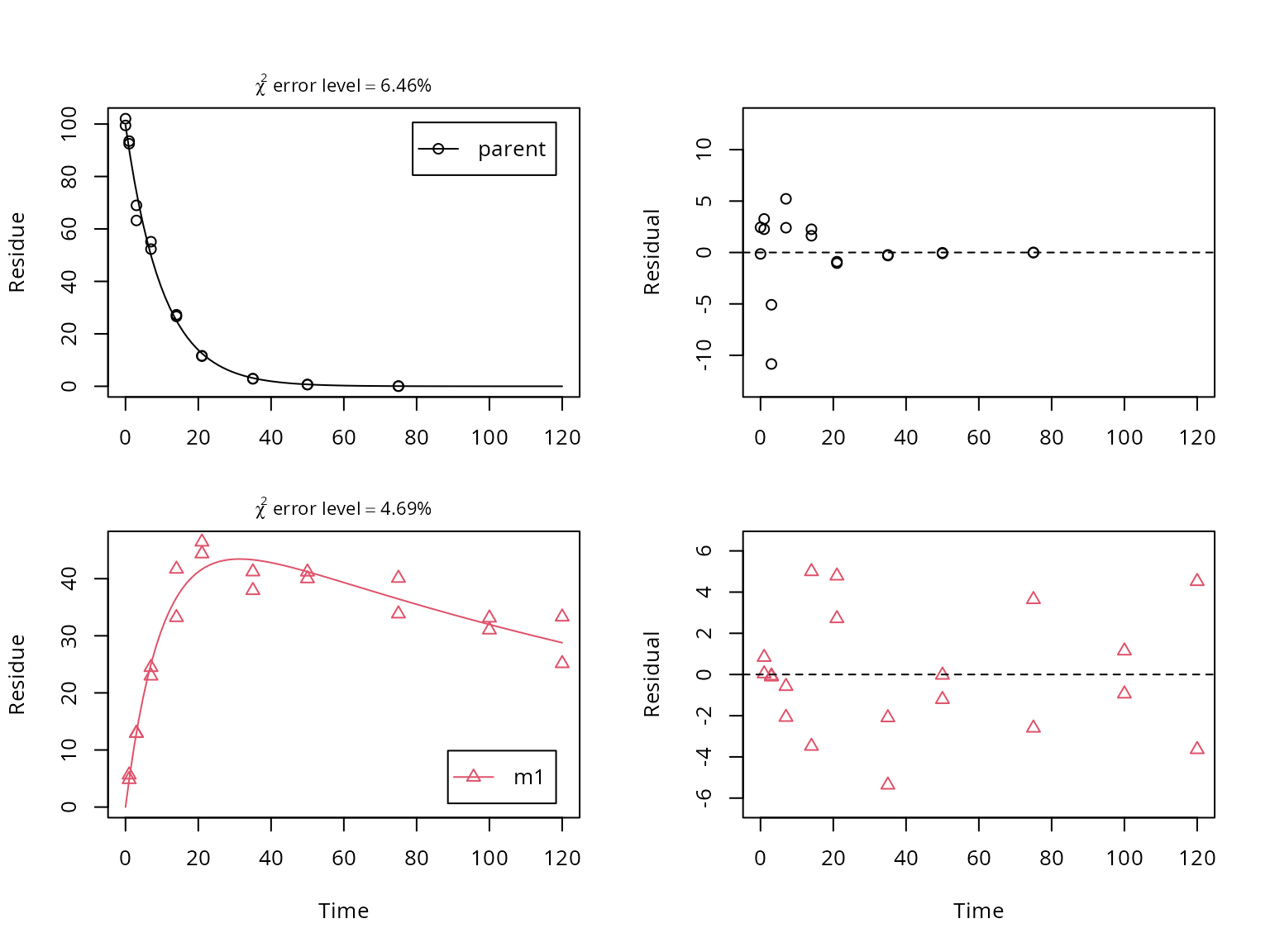
fit <- mkinfit(SFO_SFO, FOCUS_2006_D, quiet = TRUE)## Warning in mkinfit(SFO_SFO, FOCUS_2006_D, quiet = TRUE): Observations with
## value of zero were removed from the dataA plot of the fit including a residual plot for both observed
variables is obtained using the plot_sep method for
mkinfit objects, which shows separate graphs for all
compounds and their residuals.
Confidence intervals for the parameter estimates are obtained using
the mkinparplot function.
mkinparplot(fit)
A comprehensive report of the results is obtained using the
summary method for mkinfit objects.
summary(fit)## mkin version used for fitting: 1.2.10
## R version used for fitting: 4.4.2
## Date of fit: Sun Feb 16 17:04:33 2025
## Date of summary: Sun Feb 16 17:04:33 2025
##
## Equations:
## d_parent/dt = - k_parent * parent
## d_m1/dt = + f_parent_to_m1 * k_parent * parent - k_m1 * m1
##
## Model predictions using solution type analytical
##
## Fitted using 401 model solutions performed in 0.051 s
##
## Error model: Constant variance
##
## Error model algorithm: OLS
##
## Starting values for parameters to be optimised:
## value type
## parent_0 100.7500 state
## k_parent 0.1000 deparm
## k_m1 0.1001 deparm
## f_parent_to_m1 0.5000 deparm
##
## Starting values for the transformed parameters actually optimised:
## value lower upper
## parent_0 100.750000 -Inf Inf
## log_k_parent -2.302585 -Inf Inf
## log_k_m1 -2.301586 -Inf Inf
## f_parent_qlogis 0.000000 -Inf Inf
##
## Fixed parameter values:
## value type
## m1_0 0 state
##
##
## Warning(s):
## Observations with value of zero were removed from the data
##
## Results:
##
## AIC BIC logLik
## 204.4486 212.6365 -97.22429
##
## Optimised, transformed parameters with symmetric confidence intervals:
## Estimate Std. Error Lower Upper
## parent_0 99.60000 1.57000 96.4000 102.8000
## log_k_parent -2.31600 0.04087 -2.3990 -2.2330
## log_k_m1 -5.24700 0.13320 -5.5180 -4.9770
## f_parent_qlogis 0.05792 0.08926 -0.1237 0.2395
## sigma 3.12600 0.35850 2.3960 3.8550
##
## Parameter correlation:
## parent_0 log_k_parent log_k_m1 f_parent_qlogis sigma
## parent_0 1.000e+00 5.174e-01 -1.688e-01 -5.471e-01 -1.172e-06
## log_k_parent 5.174e-01 1.000e+00 -3.263e-01 -5.426e-01 -8.479e-07
## log_k_m1 -1.688e-01 -3.263e-01 1.000e+00 7.478e-01 8.211e-07
## f_parent_qlogis -5.471e-01 -5.426e-01 7.478e-01 1.000e+00 1.305e-06
## sigma -1.172e-06 -8.479e-07 8.211e-07 1.305e-06 1.000e+00
##
## Backtransformed parameters:
## Confidence intervals for internally transformed parameters are asymmetric.
## t-test (unrealistically) based on the assumption of normal distribution
## for estimators of untransformed parameters.
## Estimate t value Pr(>t) Lower Upper
## parent_0 99.600000 63.430 2.298e-36 96.400000 1.028e+02
## k_parent 0.098700 24.470 4.955e-23 0.090820 1.073e-01
## k_m1 0.005261 7.510 6.165e-09 0.004012 6.898e-03
## f_parent_to_m1 0.514500 23.070 3.104e-22 0.469100 5.596e-01
## sigma 3.126000 8.718 2.235e-10 2.396000 3.855e+00
##
## FOCUS Chi2 error levels in percent:
## err.min n.optim df
## All data 6.398 4 15
## parent 6.459 2 7
## m1 4.690 2 8
##
## Resulting formation fractions:
## ff
## parent_m1 0.5145
## parent_sink 0.4855
##
## Estimated disappearance times:
## DT50 DT90
## parent 7.023 23.33
## m1 131.761 437.70
##
## Data:
## time variable observed predicted residual
## 0 parent 99.46 99.59848 -1.385e-01
## 0 parent 102.04 99.59848 2.442e+00
## 1 parent 93.50 90.23787 3.262e+00
## 1 parent 92.50 90.23787 2.262e+00
## 3 parent 63.23 74.07319 -1.084e+01
## 3 parent 68.99 74.07319 -5.083e+00
## 7 parent 52.32 49.91207 2.408e+00
## 7 parent 55.13 49.91207 5.218e+00
## 14 parent 27.27 25.01258 2.257e+00
## 14 parent 26.64 25.01258 1.627e+00
## 21 parent 11.50 12.53462 -1.035e+00
## 21 parent 11.64 12.53462 -8.946e-01
## 35 parent 2.85 3.14787 -2.979e-01
## 35 parent 2.91 3.14787 -2.379e-01
## 50 parent 0.69 0.71624 -2.624e-02
## 50 parent 0.63 0.71624 -8.624e-02
## 75 parent 0.05 0.06074 -1.074e-02
## 75 parent 0.06 0.06074 -7.382e-04
## 1 m1 4.84 4.80296 3.704e-02
## 1 m1 5.64 4.80296 8.370e-01
## 3 m1 12.91 13.02400 -1.140e-01
## 3 m1 12.96 13.02400 -6.400e-02
## 7 m1 22.97 25.04476 -2.075e+00
## 7 m1 24.47 25.04476 -5.748e-01
## 14 m1 41.69 36.69003 5.000e+00
## 14 m1 33.21 36.69003 -3.480e+00
## 21 m1 44.37 41.65310 2.717e+00
## 21 m1 46.44 41.65310 4.787e+00
## 35 m1 41.22 43.31313 -2.093e+00
## 35 m1 37.95 43.31313 -5.363e+00
## 50 m1 41.19 41.21832 -2.832e-02
## 50 m1 40.01 41.21832 -1.208e+00
## 75 m1 40.09 36.44704 3.643e+00
## 75 m1 33.85 36.44704 -2.597e+00
## 100 m1 31.04 31.98162 -9.416e-01
## 100 m1 33.13 31.98162 1.148e+00
## 120 m1 25.15 28.78984 -3.640e+00
## 120 m1 33.31 28.78984 4.520e+00