Testing hierarchical pathway kinetics with residue data on dimethenamid and dimethenamid-P
Johannes Ranke
Last change on 20 April 2023, last compiled on 16 Februar 2025
Source:vignettes/prebuilt/2022_dmta_pathway.rmd
2022_dmta_pathway.rmdIntroduction
The purpose of this document is to test demonstrate how nonlinear hierarchical models (NLHM) based on the parent degradation models SFO, FOMC, DFOP and HS, with parallel formation of two or more metabolites can be fitted with the mkin package.
It was assembled in the course of work package 1.2 of Project Number 173340 (Application of nonlinear hierarchical models to the kinetic evaluation of chemical degradation data) of the German Environment Agency carried out in 2022 and 2023.
The mkin package is used in version 1.2.10, which is currently under
development. It contains the test data, and the functions used in the
evaluations. The saemix package is used as a backend for
fitting the NLHM, but is also loaded to make the convergence plot
function available.
This document is processed with the knitr package, which
also provides the kable function that is used to improve
the display of tabular data in R markdown documents. For parallel
processing, the parallel package is used.
library(mkin)
library(knitr)
library(saemix)
library(parallel)
n_cores <- detectCores()

# We need to start a new cluster after defining a compiled model that is
# saved as a DLL to the user directory, therefore we define a function
# This is used again after defining the pathway model
start_cluster <- function(n_cores) {
  if (Sys.info()["sysname"] == "Windows") {
    ret <- makePSOCKcluster(n_cores)
  } else {
    ret <- makeForkCluster(n_cores)
  }
  return(ret)
}
Data
The test data are available in the mkin package as an object of class
mkindsg (mkin dataset group) under the identifier
dimethenamid_2018. The following preprocessing steps are
done in this document.
- The data available for the enantiomer dimethenamid-P (DMTAP) are renamed to have the same substance name as the data for the racemic mixture dimethenamid (DMTA). The reason for this is that no difference between their degradation behaviour was identified in the EU risk assessment.
- Unnecessary columns are discarded
- The observation times of each dataset are multiplied with the corresponding normalisation factor also available in the dataset, in order to make it possible to describe all datasets with a single set of parameters that are independent of temperature
- Finally, datasets observed in the same soil (
Elliot 1andElliot 2) are combined, resulting in dimethenamid (DMTA) data from six soils.
The following commented R code performs this preprocessing.
# Apply a function to each of the seven datasets in the mkindsg object to create a list
dmta_ds <- lapply(1:7, function(i) {
  ds_i <- dimethenamid_2018$ds[[i]]$data                     # Get a dataset
  ds_i[ds_i$name == "DMTAP", "name"] <-  "DMTA"              # Rename DMTAP to DMTA
  ds_i <- subset(ds_i, select = c("name", "time", "value")) # Select data
  ds_i$time <- ds_i$time * dimethenamid_2018$f_time_norm[i]  # Normalise time
  ds_i                                                       # Return the dataset
})

# Use dataset titles as names for the list elements
names(dmta_ds) <- sapply(dimethenamid_2018$ds, function(ds) ds$title)

# Combine data for Elliot soil to obtain a named list with six elements
dmta_ds[["Elliot"]] <- rbind(dmta_ds[["Elliot 1"]], dmta_ds[["Elliot 2"]]) #
dmta_ds[["Elliot 1"]] <- NULL
dmta_ds[["Elliot 2"]] <- NULL
The following tables show the 6 datasets.
for (ds_name in names(dmta_ds)) {
  print(
    kable(mkin_long_to_wide(dmta_ds[[ds_name]]),
      caption = paste("Dataset", ds_name),
      booktabs = TRUE, row.names = FALSE))
    cat("\n\\clearpage\n")
}| time | DMTA | M23 | M27 | M31 |
|---|---|---|---|---|
| 0 | 95.8 | NA | NA | NA |
| 0 | 98.7 | NA | NA | NA |
| 14 | 60.5 | 4.1 | 1.5 | 2.0 |
| 30 | 39.1 | 5.3 | 2.4 | 2.1 |
| 59 | 15.2 | 6.0 | 3.2 | 2.2 |
| 120 | 4.8 | 4.3 | 3.8 | 1.8 |
| 120 | 4.6 | 4.1 | 3.7 | 2.1 |
| time | DMTA | M23 | M27 | M31 |
|---|---|---|---|---|
| 0.000000 | 100.5 | NA | NA | NA |
| 0.000000 | 99.6 | NA | NA | NA |
| 1.941295 | 91.9 | 0.4 | NA | NA |
| 1.941295 | 91.3 | 0.5 | 0.3 | 0.1 |
| 6.794534 | 81.8 | 1.2 | 0.8 | 1.0 |
| 6.794534 | 82.1 | 1.3 | 0.9 | 0.9 |
| 13.589067 | 69.1 | 2.8 | 1.4 | 2.0 |
| 13.589067 | 68.0 | 2.0 | 1.4 | 2.5 |
| 27.178135 | 51.4 | 2.9 | 2.7 | 4.3 |
| 27.178135 | 51.4 | 4.9 | 2.6 | 3.2 |
| 56.297565 | 27.6 | 12.2 | 4.4 | 4.3 |
| 56.297565 | 26.8 | 12.2 | 4.7 | 4.8 |
| 86.387643 | 15.7 | 12.2 | 5.4 | 5.0 |
| 86.387643 | 15.3 | 12.0 | 5.2 | 5.1 |
| 115.507073 | 7.9 | 10.4 | 5.4 | 4.3 |
| 115.507073 | 8.1 | 11.6 | 5.4 | 4.4 |
| time | DMTA | M23 | M27 | M31 |
|---|---|---|---|---|
| 0.0000000 | 96.5 | NA | NA | NA |
| 0.0000000 | 96.8 | NA | NA | NA |
| 0.0000000 | 97.0 | NA | NA | NA |
| 0.6233856 | 82.9 | 0.7 | 1.1 | 0.3 |
| 0.6233856 | 86.7 | 0.7 | 1.1 | 0.3 |
| 0.6233856 | 87.4 | 0.2 | 0.3 | 0.1 |
| 1.8701567 | 72.8 | 2.2 | 2.6 | 0.7 |
| 1.8701567 | 69.9 | 1.8 | 2.4 | 0.6 |
| 1.8701567 | 71.9 | 1.6 | 2.3 | 0.7 |
| 4.3636989 | 51.4 | 4.1 | 5.0 | 1.3 |
| 4.3636989 | 52.9 | 4.2 | 5.9 | 1.2 |
| 4.3636989 | 48.6 | 4.2 | 4.8 | 1.4 |
| 8.7273979 | 28.5 | 7.5 | 8.5 | 2.4 |
| 8.7273979 | 27.3 | 7.1 | 8.5 | 2.1 |
| 8.7273979 | 27.5 | 7.5 | 8.3 | 2.3 |
| 13.0910968 | 14.8 | 8.4 | 9.3 | 3.3 |
| 13.0910968 | 13.4 | 6.8 | 8.7 | 2.4 |
| 13.0910968 | 14.4 | 8.0 | 9.1 | 2.6 |
| 17.4547957 | 7.7 | 7.2 | 8.6 | 4.0 |
| 17.4547957 | 7.3 | 7.2 | 8.5 | 3.6 |
| 17.4547957 | 8.1 | 6.9 | 8.9 | 3.3 |
| 26.1821936 | 2.0 | 4.9 | 8.1 | 2.1 |
| 26.1821936 | 1.5 | 4.3 | 7.7 | 1.7 |
| 26.1821936 | 1.9 | 4.5 | 7.4 | 1.8 |
| 34.9095915 | 1.3 | 3.8 | 5.9 | 1.6 |
| 34.9095915 | 1.0 | 3.1 | 6.0 | 1.6 |
| 34.9095915 | 1.1 | 3.1 | 5.9 | 1.4 |
| 43.6369893 | 0.9 | 2.7 | 5.6 | 1.8 |
| 43.6369893 | 0.7 | 2.3 | 5.2 | 1.5 |
| 43.6369893 | 0.7 | 2.1 | 5.6 | 1.3 |
| 52.3643872 | 0.6 | 1.6 | 4.3 | 1.2 |
| 52.3643872 | 0.4 | 1.1 | 3.7 | 0.9 |
| 52.3643872 | 0.5 | 1.3 | 3.9 | 1.1 |
| 74.8062674 | 0.4 | 0.4 | 2.5 | 0.5 |
| 74.8062674 | 0.3 | 0.4 | 2.4 | 0.5 |
| 74.8062674 | 0.3 | 0.3 | 2.2 | 0.3 |
| time | DMTA | M23 | M27 | M31 |
|---|---|---|---|---|
| 0.0000000 | 98.09 | NA | NA | NA |
| 0.0000000 | 98.77 | NA | NA | NA |
| 0.7678922 | 93.52 | 0.36 | 0.42 | 0.36 |
| 0.7678922 | 92.03 | 0.40 | 0.47 | 0.33 |
| 2.3036765 | 88.39 | 1.03 | 0.71 | 0.55 |
| 2.3036765 | 87.18 | 1.07 | 0.82 | 0.64 |
| 5.3752452 | 69.38 | 3.60 | 2.19 | 1.94 |
| 5.3752452 | 71.06 | 3.66 | 2.28 | 1.62 |
| 10.7504904 | 45.21 | 6.97 | 5.45 | 4.22 |
| 10.7504904 | 46.81 | 7.22 | 5.19 | 4.37 |
| 16.1257355 | 30.54 | 8.65 | 8.81 | 6.31 |
| 16.1257355 | 30.07 | 8.38 | 7.93 | 6.85 |
| 21.5009807 | 21.60 | 9.10 | 10.25 | 7.05 |
| 21.5009807 | 20.41 | 8.63 | 10.77 | 6.84 |
| 32.2514711 | 9.10 | 7.63 | 10.89 | 6.53 |
| 32.2514711 | 9.70 | 8.01 | 10.85 | 7.11 |
| 43.0019614 | 6.58 | 6.40 | 10.41 | 6.06 |
| 43.0019614 | 6.31 | 6.35 | 10.35 | 6.05 |
| 53.7524518 | 3.47 | 5.35 | 9.92 | 5.50 |
| 53.7524518 | 3.52 | 5.06 | 9.42 | 5.07 |
| 64.5029421 | 3.40 | 5.14 | 9.15 | 4.94 |
| 64.5029421 | 3.67 | 5.91 | 9.25 | 4.39 |
| 91.3791680 | 1.62 | 3.35 | 7.14 | 3.64 |
| 91.3791680 | 1.62 | 2.87 | 7.13 | 3.55 |
| time | DMTA | M23 | M27 | M31 |
|---|---|---|---|---|
| 0.0000000 | 99.33 | NA | NA | NA |
| 0.0000000 | 97.44 | NA | NA | NA |
| 0.6733938 | 93.73 | 0.18 | 0.50 | 0.47 |
| 0.6733938 | 93.77 | 0.18 | 0.83 | 0.34 |
| 2.0201814 | 87.84 | 0.52 | 1.25 | 1.00 |
| 2.0201814 | 89.82 | 0.43 | 1.09 | 0.89 |
| 4.7137565 | 71.61 | 1.19 | 3.28 | 3.58 |
| 4.7137565 | 71.42 | 1.11 | 3.24 | 3.41 |
| 9.4275131 | 45.60 | 2.26 | 7.17 | 8.74 |
| 9.4275131 | 45.42 | 1.99 | 7.91 | 8.28 |
| 14.1412696 | 31.12 | 2.81 | 10.15 | 9.67 |
| 14.1412696 | 31.68 | 2.83 | 9.55 | 8.95 |
| 18.8550262 | 23.20 | 3.39 | 12.09 | 10.34 |
| 18.8550262 | 24.13 | 3.56 | 11.89 | 10.00 |
| 28.2825393 | 9.43 | 3.49 | 13.32 | 7.89 |
| 28.2825393 | 9.82 | 3.28 | 12.05 | 8.13 |
| 37.7100523 | 7.08 | 2.80 | 10.04 | 5.06 |
| 37.7100523 | 8.64 | 2.97 | 10.78 | 5.54 |
| 47.1375654 | 4.41 | 2.42 | 9.32 | 3.79 |
| 47.1375654 | 4.78 | 2.51 | 9.62 | 4.11 |
| 56.5650785 | 4.92 | 2.22 | 8.00 | 3.11 |
| 56.5650785 | 5.08 | 1.95 | 8.45 | 2.98 |
| 80.1338612 | 2.13 | 1.28 | 5.71 | 1.78 |
| 80.1338612 | 2.23 | 0.99 | 3.33 | 1.55 |
| time | DMTA | M23 | M27 | M31 |
|---|---|---|---|---|
| 0.000000 | 97.5 | NA | NA | NA |
| 0.000000 | 100.7 | NA | NA | NA |
| 1.228478 | 86.4 | NA | NA | NA |
| 1.228478 | 88.5 | NA | NA | 1.5 |
| 3.685435 | 69.8 | 2.8 | 2.3 | 5.0 |
| 3.685435 | 77.1 | 1.7 | 2.1 | 2.4 |
| 8.599349 | 59.0 | 4.3 | 4.0 | 4.3 |
| 8.599349 | 54.2 | 5.8 | 3.4 | 5.0 |
| 17.198697 | 31.3 | 8.2 | 6.6 | 8.0 |
| 17.198697 | 33.5 | 5.2 | 6.9 | 7.7 |
| 25.798046 | 19.6 | 5.1 | 8.2 | 7.8 |
| 25.798046 | 20.9 | 6.1 | 8.8 | 6.5 |
| 34.397395 | 13.3 | 6.0 | 9.7 | 8.0 |
| 34.397395 | 15.8 | 6.0 | 8.8 | 7.4 |
| 51.596092 | 6.7 | 5.0 | 8.3 | 6.9 |
| 51.596092 | 8.7 | 4.2 | 9.2 | 9.0 |
| 68.794789 | 8.8 | 3.9 | 9.3 | 5.5 |
| 68.794789 | 8.7 | 2.9 | 8.5 | 6.1 |
| 103.192184 | 6.0 | 1.9 | 8.6 | 6.1 |
| 103.192184 | 4.4 | 1.5 | 6.0 | 4.0 |
| 146.188928 | 3.3 | 2.0 | 5.6 | 3.1 |
| 146.188928 | 2.8 | 2.3 | 4.5 | 2.9 |
| 223.583066 | 1.4 | 1.2 | 4.1 | 1.8 |
| 223.583066 | 1.8 | 1.9 | 3.9 | 2.6 |
| 0.000000 | 93.4 | NA | NA | NA |
| 0.000000 | 103.2 | NA | NA | NA |
| 1.228478 | 89.2 | NA | NA | 1.3 |
| 1.228478 | 86.6 | NA | NA | NA |
| 3.685435 | 78.2 | 2.6 | 1.0 | 3.1 |
| 3.685435 | 78.1 | 2.4 | 2.6 | 2.3 |
| 8.599349 | 55.6 | 5.5 | 4.5 | 3.4 |
| 8.599349 | 53.0 | 5.6 | 4.6 | 4.3 |
| 17.198697 | 33.7 | 7.3 | 7.6 | 7.8 |
| 17.198697 | 33.2 | 6.5 | 6.7 | 8.7 |
| 25.798046 | 20.9 | 5.8 | 8.7 | 7.7 |
| 25.798046 | 19.9 | 7.7 | 7.6 | 6.5 |
| 34.397395 | 18.2 | 7.8 | 8.0 | 6.3 |
| 34.397395 | 12.7 | 7.3 | 8.6 | 8.7 |
| 51.596092 | 7.8 | 7.0 | 7.4 | 5.7 |
| 51.596092 | 9.0 | 6.3 | 7.2 | 4.2 |
| 68.794789 | 11.4 | 4.3 | 10.3 | 3.2 |
| 68.794789 | 9.0 | 3.8 | 9.4 | 4.2 |
| 103.192184 | 3.9 | 2.6 | 6.5 | 3.8 |
| 103.192184 | 4.4 | 2.8 | 6.9 | 4.0 |
| 146.188928 | 2.6 | 1.6 | 4.6 | 4.5 |
| 146.188928 | 3.4 | 1.1 | 4.5 | 4.5 |
| 223.583066 | 2.0 | 1.4 | 4.3 | 3.8 |
| 223.583066 | 1.7 | 1.3 | 4.2 | 2.3 |
Separate evaluations
As a first step to obtain suitable starting parameters for the NLHM fits, we do separate fits of several variants of the pathway model used previously (Ranke et al. 2021), varying the kinetic model for the parent compound. Because the SFORB model often provides faster convergence than the DFOP model, and can sometimes be fitted where the DFOP model results in errors, it is included in the set of parent models tested here.
if (!dir.exists("dmta_dlls")) dir.create("dmta_dlls")
m_sfo_path_1 <- mkinmod(
  DMTA = mkinsub("SFO", c("M23", "M27", "M31")),
  M23 = mkinsub("SFO"),
  M27 = mkinsub("SFO"),
  M31 = mkinsub("SFO", "M27", sink = FALSE),
  name = "m_sfo_path", dll_dir = "dmta_dlls",
  unload = TRUE, overwrite = TRUE,
  quiet = TRUE
)
m_fomc_path_1 <- mkinmod(
  DMTA = mkinsub("FOMC", c("M23", "M27", "M31")),
  M23 = mkinsub("SFO"),
  M27 = mkinsub("SFO"),
  M31 = mkinsub("SFO", "M27", sink = FALSE),
  name = "m_fomc_path", dll_dir = "dmta_dlls",
  unload = TRUE, overwrite = TRUE,
  quiet = TRUE
)
m_dfop_path_1 <- mkinmod(
  DMTA = mkinsub("DFOP", c("M23", "M27", "M31")),
  M23 = mkinsub("SFO"),
  M27 = mkinsub("SFO"),
  M31 = mkinsub("SFO", "M27", sink = FALSE),
  name = "m_dfop_path", dll_dir = "dmta_dlls",
  unload = TRUE, overwrite = TRUE,
  quiet = TRUE
)
m_sforb_path_1 <- mkinmod(
  DMTA = mkinsub("SFORB", c("M23", "M27", "M31")),
  M23 = mkinsub("SFO"),
  M27 = mkinsub("SFO"),
  M31 = mkinsub("SFO", "M27", sink = FALSE),
  name = "m_sforb_path", dll_dir = "dmta_dlls",
  unload = TRUE, overwrite = TRUE,
  quiet = TRUE
)
m_hs_path_1 <- mkinmod(
  DMTA = mkinsub("HS", c("M23", "M27", "M31")),
  M23 = mkinsub("SFO"),
  M27 = mkinsub("SFO"),
  M31 = mkinsub("SFO", "M27", sink = FALSE),
  name = "m_hs_path", dll_dir = "dmta_dlls",
  unload = TRUE, overwrite = TRUE,
  quiet = TRUE
)
cl <- start_cluster(n_cores)

deg_mods_1 <- list(
  sfo_path_1 = m_sfo_path_1,
  fomc_path_1 = m_fomc_path_1,
  dfop_path_1 = m_dfop_path_1,
  sforb_path_1 = m_sforb_path_1,
  hs_path_1 = m_hs_path_1)

sep_1_const <- mmkin(
  deg_mods_1,
  dmta_ds,
  error_model = "const",
  quiet = TRUE)

status(sep_1_const) |> kable()| Calke | Borstel | Flaach | BBA 2.2 | BBA 2.3 | Elliot | |
|---|---|---|---|---|---|---|
| sfo_path_1 | OK | OK | OK | OK | OK | OK |
| fomc_path_1 | OK | OK | OK | OK | OK | OK |
| dfop_path_1 | OK | OK | OK | OK | OK | OK |
| sforb_path_1 | OK | OK | C | OK | OK | OK |
| hs_path_1 | C | C | OK | C | C | C |
All separate pathway fits with SFO or FOMC for the parent and constant variance converged (status OK). Most fits with DFOP or SFORB for the parent converged as well. The fits with HS for the parent did not converge with default settings.
| Calke | Borstel | Flaach | BBA 2.2 | BBA 2.3 | Elliot | |
|---|---|---|---|---|---|---|
| sfo_path_1 | OK | OK | OK | OK | OK | OK |
| fomc_path_1 | OK | OK | OK | OK | OK | OK |
| dfop_path_1 | OK | C | OK | C | OK | OK |
| sforb_path_1 | OK | OK | OK | OK | OK | OK |
| hs_path_1 | C | C | C | C | C | C |
With the two-component error model, the set of fits with convergence problems is slightly different, with convergence problems appearing for different data sets when applying the DFOP and SFORB model and some additional convergence problems when using the FOMC model for the parent.
Hierarchichal model fits
The following code fits two sets of the corresponding hierarchical models to the data, one assuming constant variance, and one assuming two-component error.
The run time for these fits was around two hours on five year old hardware. After a recent hardware upgrade these fits complete in less than twenty minutes.
| const | tc | |
|---|---|---|
| sfo_path_1 | OK | OK |
| fomc_path_1 | OK | OK |
| dfop_path_1 | OK | OK |
| sforb_path_1 | OK | OK |
| hs_path_1 | OK | OK |
According to the status function, all fits terminated
successfully.
| npar | AIC | BIC | Lik | |
|---|---|---|---|---|
| sfo_path_1 const | 17 | 2291.8 | 2288.3 | -1128.9 |
| sfo_path_1 tc | 18 | 2276.4 | 2272.7 | -1120.2 |
| fomc_path_1 const | 19 | 2095.9 | 2091.9 | -1028.9 |
| fomc_path_1 tc | 20 | 1939.0 | 1934.8 | -949.5 |
| dfop_path_1 const | 21 | 2039.7 | 2035.3 | -998.8 |
| sforb_path_1 const | 21 | 2017.7 | 2013.4 | -987.9 |
| hs_path_1 const | 21 | 2023.7 | 2019.3 | -990.9 |
| dfop_path_1 tc | 22 | 1881.7 | 1877.1 | -918.9 |
| sforb_path_1 tc | 22 | 1832.7 | 1828.1 | -894.3 |
| hs_path_1 tc | 22 | 1831.6 | 1827.0 | -893.8 |
When the goodness-of-fit of the models is compared, a warning is obtained, indicating that the likelihood of the pathway fit with SFORB for the parent compound and constant variance could not be calculated with importance sampling (method ‘is’). As this is the default method on which all AIC and BIC comparisons are based, this variant is not included in the model comparison table. Comparing the goodness-of-fit of the remaining models, HS model model with two-component error provides the best fit. However, for batch experiments performed with constant conditions such as the experiments evaluated here, there is no reason to assume a discontinuity, so the SFORB model is preferable from a mechanistic viewpoint. In addition, the information criteria AIC and BIC are very similar for HS and SFORB. Therefore, the SFORB model is selected here for further refinements.
Parameter identifiability based on the Fisher Information Matrix
Using the illparms function, ill-defined statistical
model parameters such as standard deviations of the degradation
parameters in the population and error model parameters can be
found.
| const | tc | |
|---|---|---|
| sfo_path_1 | sd(DMTA_0) | |
| fomc_path_1 | sd(DMTA_0) | |
| dfop_path_1 | ||
| sforb_path_1 | sd(log_k_DMTA_bound_free) | sd(log_k_DMTA_bound_free) |
| hs_path_1 | sd(log_tb) |
When using constant variance, no ill-defined variance parameters are
identified with the illparms function in any of the
degradation models. When using the two-component error model, there is
one ill-defined variance parameter in all variants except for the
variant using DFOP for the parent compound.
For the selected combination of the SFORB pathway model with
two-component error, the random effect for the rate constant from
reversibly bound DMTA to the free DMTA (k_DMTA_bound_free)
is not well-defined. Therefore, the fit is updated without assuming a
random effect for this parameter.
saem_sforb_path_1_tc_reduced <- update(saem_1[["sforb_path_1", "tc"]],
  no_random_effect = "log_k_DMTA_bound_free")
illparms(saem_sforb_path_1_tc_reduced)
As expected, no ill-defined parameters remain. The model comparison below shows that the reduced model is preferable.
| npar | AIC | BIC | Lik | |
|---|---|---|---|---|
| saem_sforb_path_1_tc_reduced | 21 | 1830.4 | 1826.0 | -894.2 |
| saem_1[[“sforb_path_1”, “tc”]] | 22 | 1832.7 | 1828.1 | -894.3 |
The convergence plot of the refined fit is shown below.
plot(saem_sforb_path_1_tc_reduced$so, plot.type = "convergence")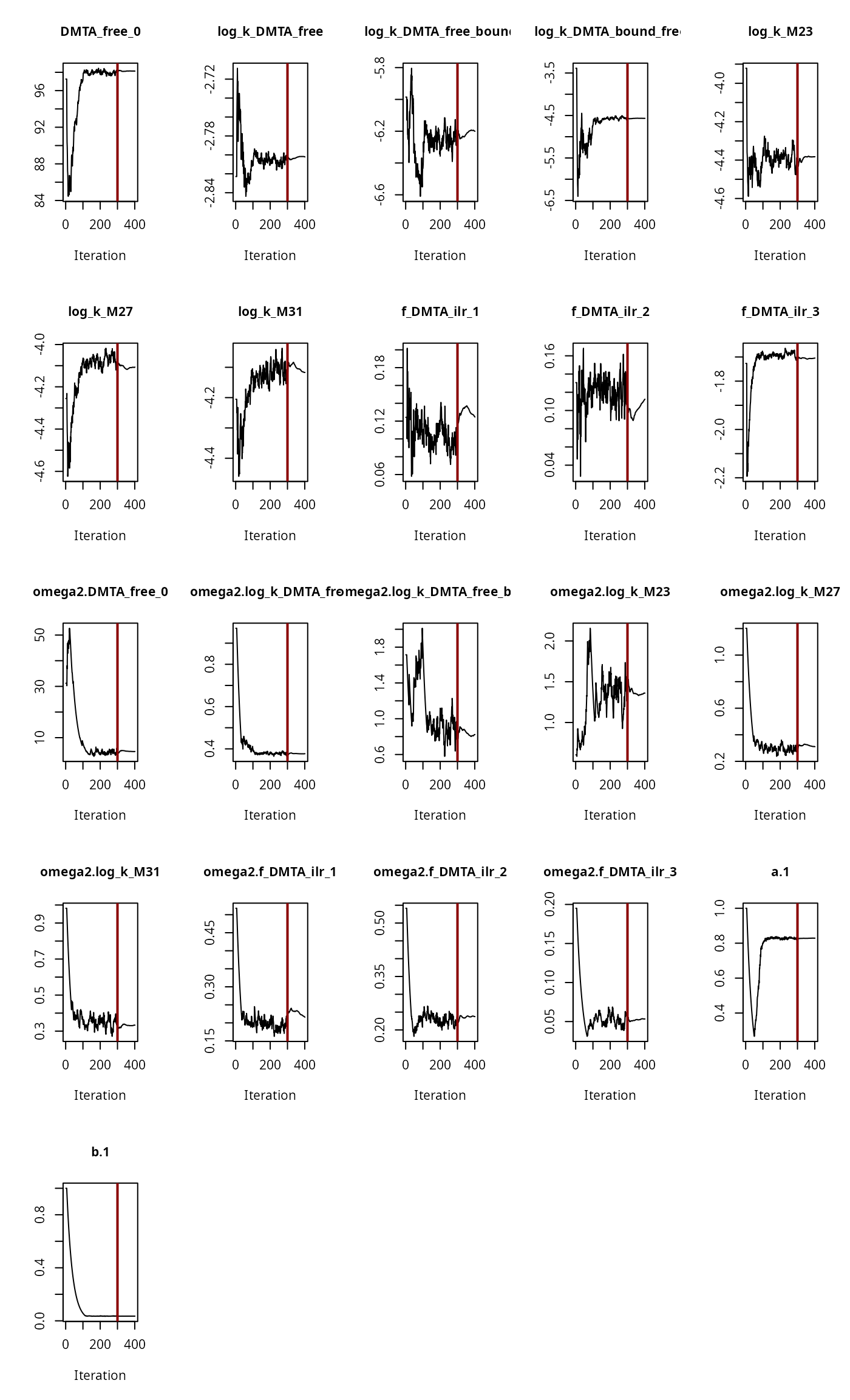
For some parameters, for example for f_DMTA_ilr_1 and
f_DMTA_ilr_2, i.e. for two of the parameters determining
the formation fractions of the parallel formation of the three
metabolites, some movement of the parameters is still visible in the
second phase of the algorithm. However, the amplitude of this movement
is in the range of the amplitude towards the end of the first phase.
Therefore, it is likely that an increase in iterations would not improve
the parameter estimates very much, and it is proposed that the fit is
acceptable. No numeric convergence criterion is implemented in
saemix.
Alternative check of parameter identifiability
As an alternative check of parameter identifiability (Duchesne et al. 2021), multistart runs were performed on the basis of the refined fit shown above.
saem_sforb_path_1_tc_reduced_multi <- multistart(saem_sforb_path_1_tc_reduced,
  n = 32, cores = 10)
(subscript) logical subscript too long
print(saem_sforb_path_1_tc_reduced_multi)<multistart> object with 32 fits:
E OK
7 25
OK: Fit terminated successfully
E: ErrorOut of the 32 fits that were initiated, only 17 terminated without an error. The reason for this is that the wide variation of starting parameters in combination with the parameter variation that is used in the SAEM algorithm leads to parameter combinations for the degradation model that the numerical integration routine cannot cope with. Because of this variation of initial parameters, some of the model fits take up to two times more time than the original fit.
par(mar = c(12.1, 4.1, 2.1, 2.1))
parplot(saem_sforb_path_1_tc_reduced_multi, ylim = c(0.5, 2), las = 2)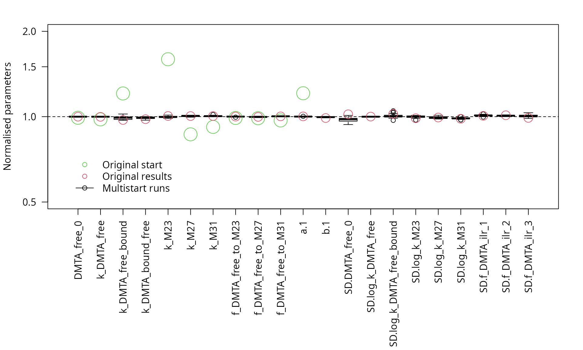
Parameter boxplots for the multistart runs that succeeded
However, visual analysis of the boxplot of the parameters obtained in the successful fits confirms that the results are sufficiently independent of the starting parameters, and there are no remaining ill-defined parameters.
Plots of selected fits
The SFORB pathway fits with full and reduced parameter distribution model are shown below.
plot(saem_1[["sforb_path_1", "tc"]])
SFORB pathway fit with two-component error
plot(saem_sforb_path_1_tc_reduced)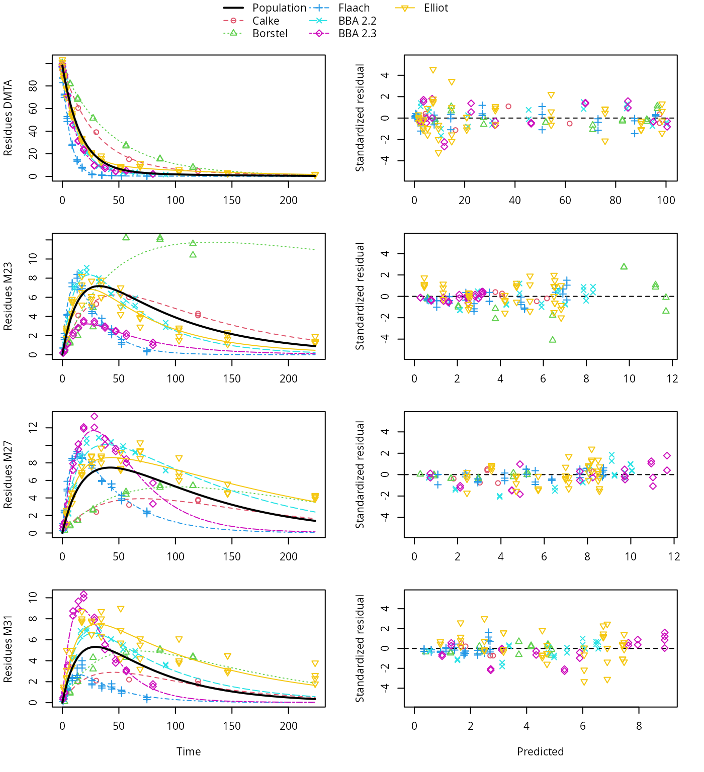
SFORB pathway fit with two-component error, reduced parameter model
Plots of the remaining fits and listings for all successful fits are shown in the Appendix.
stopCluster(cl)Conclusions
Pathway fits with SFO, FOMC, DFOP, SFORB and HS models for the parent compound could be successfully performed.
Acknowledgements
The helpful comments by Janina Wöltjen of the German Environment Agency on earlier versions of this document are gratefully acknowledged.
References
Appendix
Plots of hierarchical fits not selected for refinement
plot(saem_1[["sfo_path_1", "tc"]])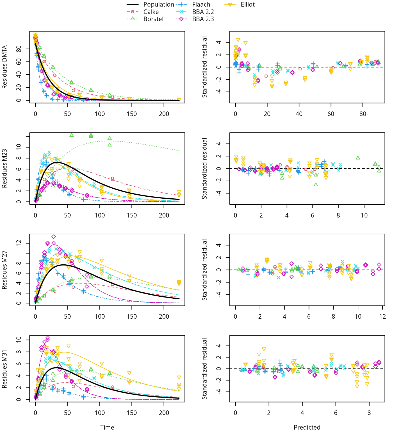
SFO pathway fit with two-component error
plot(saem_1[["fomc_path_1", "tc"]])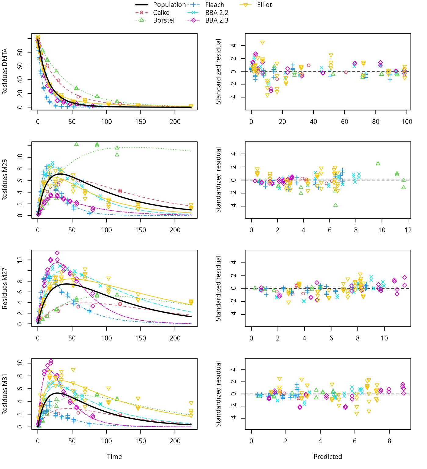
FOMC pathway fit with two-component error
plot(saem_1[["sforb_path_1", "tc"]])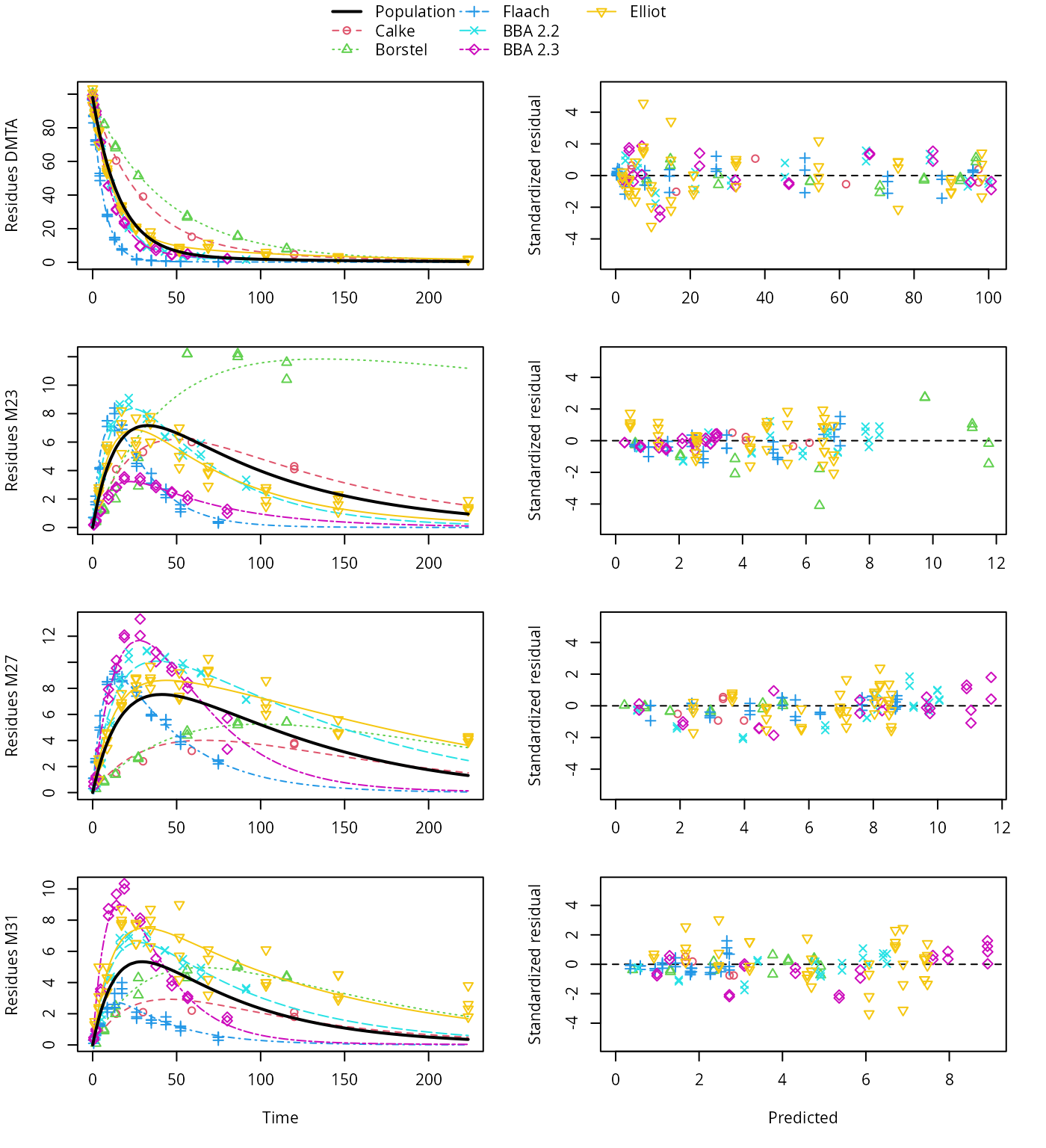
HS pathway fit with two-component error
Session info
R version 4.4.2 (2024-10-31)
Platform: x86_64-pc-linux-gnu
Running under: Debian GNU/Linux 12 (bookworm)

Matrix products: default
BLAS:   /usr/lib/x86_64-linux-gnu/blas/libblas.so.3.11.0
LAPACK: /usr/lib/x86_64-linux-gnu/lapack/liblapack.so.3.11.0

locale:
 [1] LC_CTYPE=de_DE.UTF-8       LC_NUMERIC=C
 [3] LC_TIME=de_DE.UTF-8        LC_COLLATE=de_DE.UTF-8
 [5] LC_MONETARY=de_DE.UTF-8    LC_MESSAGES=de_DE.UTF-8
 [7] LC_PAPER=de_DE.UTF-8       LC_NAME=C
 [9] LC_ADDRESS=C               LC_TELEPHONE=C
[11] LC_MEASUREMENT=de_DE.UTF-8 LC_IDENTIFICATION=C

time zone: Europe/Berlin
tzcode source: system (glibc)

attached base packages:
[1] parallel  stats     graphics  grDevices utils     datasets  methods
[8] base

other attached packages:
[1] rmarkdown_2.29  nvimcom_0.9-167 saemix_3.3      npde_3.5
[5] knitr_1.49      mkin_1.2.10

loaded via a namespace (and not attached):
 [1] sass_0.4.9        utf8_1.2.4        generics_0.1.3    lattice_0.22-6
 [5] digest_0.6.37     magrittr_2.0.3    evaluate_1.0.1    grid_4.4.2
 [9] fastmap_1.2.0     jsonlite_1.8.9    processx_3.8.4    pkgbuild_1.4.5
[13] deSolve_1.40      mclust_6.1.1      ps_1.8.1          gridExtra_2.3
[17] fansi_1.0.6       scales_1.3.0      codetools_0.2-20  textshaping_0.4.1
[21] jquerylib_0.1.4   cli_3.6.3         rlang_1.1.4       munsell_0.5.1
[25] cachem_1.1.0      yaml_2.3.10       inline_0.3.20     tools_4.4.2
[29] dplyr_1.1.4       colorspace_2.1-1  ggplot2_3.5.1     vctrs_0.6.5
[33] R6_2.5.1          zoo_1.8-12        lifecycle_1.0.4   fs_1.6.5
[37] htmlwidgets_1.6.4 MASS_7.3-61       ragg_1.3.3        pkgconfig_2.0.3
[41] desc_1.4.3        callr_3.7.6       pkgdown_2.1.1     pillar_1.9.0
[45] bslib_0.8.0       gtable_0.3.6      glue_1.8.0        systemfonts_1.1.0
[49] xfun_0.49         tibble_3.2.1      lmtest_0.9-40     tidyselect_1.2.1
[53] htmltools_0.5.8.1 nlme_3.1-166      compiler_4.4.2