This function uses saemix::saemix() as a backend for fitting nonlinear mixed
effects models created from mmkin row objects using the Stochastic Approximation
Expectation Maximisation algorithm (SAEM).
Usage
saem(object, ...)

# S3 method for class 'mmkin'
saem(
  object,
  transformations = c("mkin", "saemix"),
  error_model = "auto",
  degparms_start = numeric(),
  test_log_parms = TRUE,
  conf.level = 0.6,
  solution_type = "auto",
  covariance.model = "auto",
  omega.init = "auto",
  covariates = NULL,
  covariate_models = NULL,
  no_random_effect = NULL,
  error.init = c(1, 1),
  nbiter.saemix = c(300, 100),
  control = list(displayProgress = FALSE, print = FALSE, nbiter.saemix = nbiter.saemix,
    save = FALSE, save.graphs = FALSE),
  verbose = FALSE,
  quiet = FALSE,
  ...
)

# S3 method for class 'saem.mmkin'
print(x, digits = max(3, getOption("digits") - 3), ...)

saemix_model(
  object,
  solution_type = "auto",
  transformations = c("mkin", "saemix"),
  error_model = "auto",
  degparms_start = numeric(),
  covariance.model = "auto",
  no_random_effect = NULL,
  omega.init = "auto",
  covariates = NULL,
  covariate_models = NULL,
  error.init = numeric(),
  test_log_parms = FALSE,
  conf.level = 0.6,
  verbose = FALSE,
  ...
)

saemix_data(object, covariates = NULL, verbose = FALSE, ...)
Arguments
- object
An mmkin row object containing several fits of the same mkinmod model to different datasets
- ...
Further parameters passed to saemix::saemixModel.
- transformations
Per default, all parameter transformations are done in mkin. If this argument is set to 'saemix', parameter transformations are done in 'saemix' for the supported cases, i.e. (as of version 1.1.2) SFO, FOMC, DFOP and HS without fixing
parent_0, and SFO or DFOP with one SFO metabolite.- error_model
Possibility to override the error model used in the mmkin object
- degparms_start
Parameter values given as a named numeric vector will be used to override the starting values obtained from the 'mmkin' object.
- test_log_parms
If TRUE, an attempt is made to use more robust starting values for population parameters fitted as log parameters in mkin (like rate constants) by only considering rate constants that pass the t-test when calculating mean degradation parameters using mean_degparms.
- conf.level
Possibility to adjust the required confidence level for parameter that are tested if requested by 'test_log_parms'.
- solution_type
Possibility to specify the solution type in case the automatic choice is not desired
- covariance.model
Will be passed to
saemix::saemixModel(). Per default, uncorrelated random effects are specified for all degradation parameters.- omega.init
Will be passed to
saemix::saemixModel(). If using mkin transformations and the default covariance model with optionally excluded random effects, the variances of the degradation parameters are estimated using mean_degparms, with testing of untransformed log parameters for significant difference from zero. If not using mkin transformations or a custom covariance model, the default initialisation of saemix::saemixModel is used for omega.init.- covariates
A data frame with covariate data for use in 'covariate_models', with dataset names as row names.
- covariate_models
A list containing linear model formulas with one explanatory variable, i.e. of the type 'parameter ~ covariate'. Covariates must be available in the 'covariates' data frame.
- no_random_effect
Character vector of degradation parameters for which there should be no variability over the groups. Only used if the covariance model is not explicitly specified.
- error.init
Will be passed to
saemix::saemixModel().- nbiter.saemix
Convenience option to increase the number of iterations
- control
Passed to saemix::saemix.
- verbose
Should we print information about created objects of type saemix::SaemixModel and saemix::SaemixData?
- quiet
Should we suppress the messages saemix prints at the beginning and the end of the optimisation process?
- x
An saem.mmkin object to print
- digits
Number of digits to use for printing
Value
An S3 object of class 'saem.mmkin', containing the fitted saemix::SaemixObject as a list component named 'so'. The object also inherits from 'mixed.mmkin'.
An saemix::SaemixModel object.
An saemix::SaemixData object.
Details
An mmkin row object is essentially a list of mkinfit objects that have been obtained by fitting the same model to a list of datasets using mkinfit.
Starting values for the fixed effects (population mean parameters, argument
psi0 of saemix::saemixModel() are the mean values of the parameters found
using mmkin.
Examples
# \dontrun{
ds <- lapply(experimental_data_for_UBA_2019[6:10],
function(x) subset(x$data[c("name", "time", "value")]))
names(ds) <- paste("Dataset", 6:10)
f_mmkin_parent_p0_fixed <- mmkin("FOMC", ds,
state.ini = c(parent = 100), fixed_initials = "parent", quiet = TRUE)
f_saem_p0_fixed <- saem(f_mmkin_parent_p0_fixed)
f_mmkin_parent <- mmkin(c("SFO", "FOMC", "DFOP"), ds, quiet = TRUE)
f_saem_sfo <- saem(f_mmkin_parent["SFO", ])
f_saem_fomc <- saem(f_mmkin_parent["FOMC", ])
f_saem_dfop <- saem(f_mmkin_parent["DFOP", ])
anova(f_saem_sfo, f_saem_fomc, f_saem_dfop)
#> Data: 90 observations of 1 variable(s) grouped in 5 datasets
#>
#> npar AIC BIC Lik
#> f_saem_sfo 5 624.33 622.38 -307.17
#> f_saem_fomc 7 467.85 465.11 -226.92
#> f_saem_dfop 9 493.76 490.24 -237.88
anova(f_saem_sfo, f_saem_dfop, test = TRUE)
#> Data: 90 observations of 1 variable(s) grouped in 5 datasets
#>
#> npar AIC BIC Lik Chisq Df Pr(>Chisq)
#> f_saem_sfo 5 624.33 622.38 -307.17
#> f_saem_dfop 9 493.76 490.24 -237.88 138.57 4 < 2.2e-16 ***
#> ---
#> Signif. codes: 0 ‘***’ 0.001 ‘**’ 0.01 ‘*’ 0.05 ‘.’ 0.1 ‘ ’ 1
illparms(f_saem_dfop)
#> [1] "sd(g_qlogis)"
f_saem_dfop_red <- update(f_saem_dfop, no_random_effect = "g_qlogis")
anova(f_saem_dfop, f_saem_dfop_red, test = TRUE)
#> Data: 90 observations of 1 variable(s) grouped in 5 datasets
#>
#> npar AIC BIC Lik Chisq Df Pr(>Chisq)
#> f_saem_dfop_red 8 488.68 485.55 -236.34
#> f_saem_dfop 9 493.76 490.24 -237.88 0 1 1
anova(f_saem_sfo, f_saem_fomc, f_saem_dfop)
#> Data: 90 observations of 1 variable(s) grouped in 5 datasets
#>
#> npar AIC BIC Lik
#> f_saem_sfo 5 624.33 622.38 -307.17
#> f_saem_fomc 7 467.85 465.11 -226.92
#> f_saem_dfop 9 493.76 490.24 -237.88
# The returned saem.mmkin object contains an SaemixObject, therefore we can use
# functions from saemix
library(saemix)
#> Loading required package: npde
#> Package saemix, version 3.3, March 2024
#> please direct bugs, questions and feedback to emmanuelle.comets@inserm.fr
#>
#> Attaching package: ‘saemix’
#> The following objects are masked from ‘package:npde’:
#>
#> kurtosis, skewness
compare.saemix(f_saem_sfo$so, f_saem_fomc$so, f_saem_dfop$so)
#> Likelihoods calculated by importance sampling
#> AIC BIC
#> 1 624.3316 622.3788
#> 2 467.8472 465.1132
#> 3 493.7592 490.2441
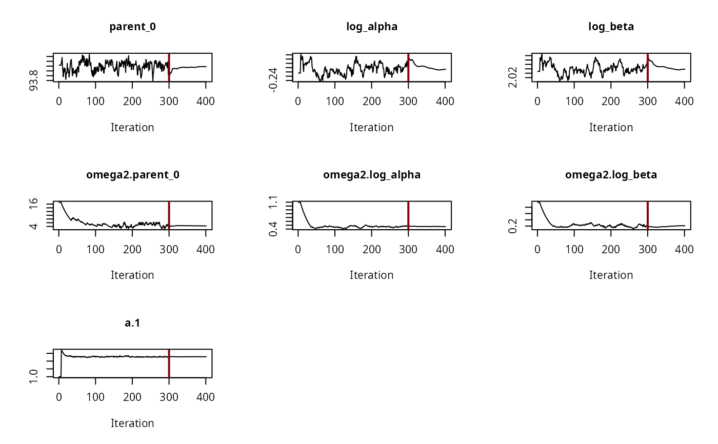
plot(f_saem_fomc$so, plot.type = "convergence")
 plot(f_saem_fomc$so, plot.type = "individual.fit")
#> Simulating data using nsim = 1000 simulated datasets
#> Computing WRES and npde .
plot(f_saem_fomc$so, plot.type = "individual.fit")
#> Simulating data using nsim = 1000 simulated datasets
#> Computing WRES and npde .
 plot(f_saem_fomc$so, plot.type = "npde")
#> Simulating data using nsim = 1000 simulated datasets
#> Computing WRES and npde .
#> Please use npdeSaemix to obtain VPC and npde
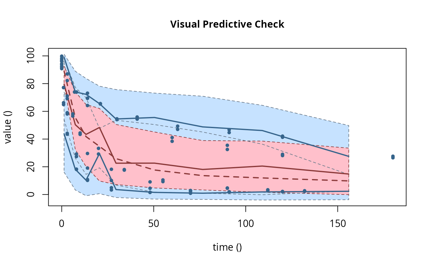
plot(f_saem_fomc$so, plot.type = "vpc")
plot(f_saem_fomc$so, plot.type = "npde")
#> Simulating data using nsim = 1000 simulated datasets
#> Computing WRES and npde .
#> Please use npdeSaemix to obtain VPC and npde
plot(f_saem_fomc$so, plot.type = "vpc")
 f_mmkin_parent_tc <- update(f_mmkin_parent, error_model = "tc")
f_saem_fomc_tc <- saem(f_mmkin_parent_tc["FOMC", ])
anova(f_saem_fomc, f_saem_fomc_tc, test = TRUE)
#> Data: 90 observations of 1 variable(s) grouped in 5 datasets
#>
#> npar AIC BIC Lik Chisq Df Pr(>Chisq)
#> f_saem_fomc 7 467.85 465.11 -226.92
#> f_saem_fomc_tc 8 469.90 466.77 -226.95 0 1 1
sfo_sfo <- mkinmod(parent = mkinsub("SFO", "A1"),
A1 = mkinsub("SFO"))
#> Temporary DLL for differentials generated and loaded
fomc_sfo <- mkinmod(parent = mkinsub("FOMC", "A1"),
A1 = mkinsub("SFO"))
#> Temporary DLL for differentials generated and loaded
dfop_sfo <- mkinmod(parent = mkinsub("DFOP", "A1"),
A1 = mkinsub("SFO"))
#> Temporary DLL for differentials generated and loaded
# The following fit uses analytical solutions for SFO-SFO and DFOP-SFO,
# and compiled ODEs for FOMC that are much slower
f_mmkin <- mmkin(list(
"SFO-SFO" = sfo_sfo, "FOMC-SFO" = fomc_sfo, "DFOP-SFO" = dfop_sfo),
ds, quiet = TRUE)
# saem fits of SFO-SFO and DFOP-SFO to these data take about five seconds
# each on this system, as we use analytical solutions written for saemix.
# When using the analytical solutions written for mkin this took around
# four minutes
f_saem_sfo_sfo <- saem(f_mmkin["SFO-SFO", ])
f_saem_dfop_sfo <- saem(f_mmkin["DFOP-SFO", ])
# We can use print, plot and summary methods to check the results
print(f_saem_dfop_sfo)
#> Kinetic nonlinear mixed-effects model fit by SAEM
#> Structural model:
#> d_parent/dt = - ((k1 * g * exp(-k1 * time) + k2 * (1 - g) * exp(-k2 *
#> time)) / (g * exp(-k1 * time) + (1 - g) * exp(-k2 * time)))
#> * parent
#> d_A1/dt = + f_parent_to_A1 * ((k1 * g * exp(-k1 * time) + k2 * (1 - g)
#> * exp(-k2 * time)) / (g * exp(-k1 * time) + (1 - g) *
#> exp(-k2 * time))) * parent - k_A1 * A1
#>
#> Data:
#> 170 observations of 2 variable(s) grouped in 5 datasets
#>
#> Likelihood computed by importance sampling
#> AIC BIC logLik
#> 839.2 834.1 -406.6
#>
#> Fitted parameters:
#> estimate lower upper
#> parent_0 93.70402 91.04104 96.3670
#> log_k_A1 -5.83760 -7.66452 -4.0107
#> f_parent_qlogis -0.95718 -1.35955 -0.5548
#> log_k1 -2.35514 -3.39402 -1.3163
#> log_k2 -3.79634 -5.64009 -1.9526
#> g_qlogis -0.02108 -0.66463 0.6225
#> a.1 1.88191 1.66491 2.0989
#> SD.parent_0 2.81628 0.78922 4.8433
#> SD.log_k_A1 1.78751 0.42105 3.1540
#> SD.f_parent_qlogis 0.45016 0.16116 0.7391
#> SD.log_k1 1.06923 0.31676 1.8217
#> SD.log_k2 2.03768 0.70938 3.3660
#> SD.g_qlogis 0.44024 -0.09262 0.9731
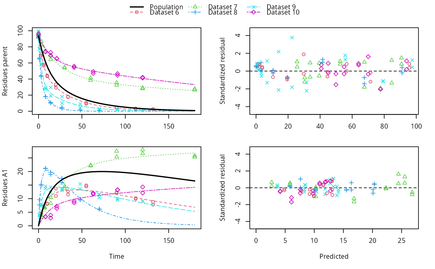
plot(f_saem_dfop_sfo)
f_mmkin_parent_tc <- update(f_mmkin_parent, error_model = "tc")
f_saem_fomc_tc <- saem(f_mmkin_parent_tc["FOMC", ])
anova(f_saem_fomc, f_saem_fomc_tc, test = TRUE)
#> Data: 90 observations of 1 variable(s) grouped in 5 datasets
#>
#> npar AIC BIC Lik Chisq Df Pr(>Chisq)
#> f_saem_fomc 7 467.85 465.11 -226.92
#> f_saem_fomc_tc 8 469.90 466.77 -226.95 0 1 1
sfo_sfo <- mkinmod(parent = mkinsub("SFO", "A1"),
A1 = mkinsub("SFO"))
#> Temporary DLL for differentials generated and loaded
fomc_sfo <- mkinmod(parent = mkinsub("FOMC", "A1"),
A1 = mkinsub("SFO"))
#> Temporary DLL for differentials generated and loaded
dfop_sfo <- mkinmod(parent = mkinsub("DFOP", "A1"),
A1 = mkinsub("SFO"))
#> Temporary DLL for differentials generated and loaded
# The following fit uses analytical solutions for SFO-SFO and DFOP-SFO,
# and compiled ODEs for FOMC that are much slower
f_mmkin <- mmkin(list(
"SFO-SFO" = sfo_sfo, "FOMC-SFO" = fomc_sfo, "DFOP-SFO" = dfop_sfo),
ds, quiet = TRUE)
# saem fits of SFO-SFO and DFOP-SFO to these data take about five seconds
# each on this system, as we use analytical solutions written for saemix.
# When using the analytical solutions written for mkin this took around
# four minutes
f_saem_sfo_sfo <- saem(f_mmkin["SFO-SFO", ])
f_saem_dfop_sfo <- saem(f_mmkin["DFOP-SFO", ])
# We can use print, plot and summary methods to check the results
print(f_saem_dfop_sfo)
#> Kinetic nonlinear mixed-effects model fit by SAEM
#> Structural model:
#> d_parent/dt = - ((k1 * g * exp(-k1 * time) + k2 * (1 - g) * exp(-k2 *
#> time)) / (g * exp(-k1 * time) + (1 - g) * exp(-k2 * time)))
#> * parent
#> d_A1/dt = + f_parent_to_A1 * ((k1 * g * exp(-k1 * time) + k2 * (1 - g)
#> * exp(-k2 * time)) / (g * exp(-k1 * time) + (1 - g) *
#> exp(-k2 * time))) * parent - k_A1 * A1
#>
#> Data:
#> 170 observations of 2 variable(s) grouped in 5 datasets
#>
#> Likelihood computed by importance sampling
#> AIC BIC logLik
#> 839.2 834.1 -406.6
#>
#> Fitted parameters:
#> estimate lower upper
#> parent_0 93.70402 91.04104 96.3670
#> log_k_A1 -5.83760 -7.66452 -4.0107
#> f_parent_qlogis -0.95718 -1.35955 -0.5548
#> log_k1 -2.35514 -3.39402 -1.3163
#> log_k2 -3.79634 -5.64009 -1.9526
#> g_qlogis -0.02108 -0.66463 0.6225
#> a.1 1.88191 1.66491 2.0989
#> SD.parent_0 2.81628 0.78922 4.8433
#> SD.log_k_A1 1.78751 0.42105 3.1540
#> SD.f_parent_qlogis 0.45016 0.16116 0.7391
#> SD.log_k1 1.06923 0.31676 1.8217
#> SD.log_k2 2.03768 0.70938 3.3660
#> SD.g_qlogis 0.44024 -0.09262 0.9731
plot(f_saem_dfop_sfo)
 summary(f_saem_dfop_sfo, data = TRUE)
#> saemix version used for fitting: 3.3
#> mkin version used for pre-fitting: 1.2.10
#> R version used for fitting: 4.4.2
#> Date of fit: Sun Feb 16 17:01:05 2025
#> Date of summary: Sun Feb 16 17:01:05 2025
#>
#> Equations:
#> d_parent/dt = - ((k1 * g * exp(-k1 * time) + k2 * (1 - g) * exp(-k2 *
#> time)) / (g * exp(-k1 * time) + (1 - g) * exp(-k2 * time)))
#> * parent
#> d_A1/dt = + f_parent_to_A1 * ((k1 * g * exp(-k1 * time) + k2 * (1 - g)
#> * exp(-k2 * time)) / (g * exp(-k1 * time) + (1 - g) *
#> exp(-k2 * time))) * parent - k_A1 * A1
#>
#> Data:
#> 170 observations of 2 variable(s) grouped in 5 datasets
#>
#> Model predictions using solution type analytical
#>
#> Fitted in 3.489 s
#> Using 300, 100 iterations and 10 chains
#>
#> Variance model: Constant variance
#>
#> Starting values for degradation parameters:
#> parent_0 log_k_A1 f_parent_qlogis log_k1 log_k2
#> 93.8102 -5.3734 -0.9711 -1.8799 -4.2708
#> g_qlogis
#> 0.1356
#>
#> Fixed degradation parameter values:
#> None
#>
#> Starting values for random effects (square root of initial entries in omega):
#> parent_0 log_k_A1 f_parent_qlogis log_k1 log_k2 g_qlogis
#> parent_0 4.941 0.000 0.0000 0.000 0.000 0.0000
#> log_k_A1 0.000 2.551 0.0000 0.000 0.000 0.0000
#> f_parent_qlogis 0.000 0.000 0.7251 0.000 0.000 0.0000
#> log_k1 0.000 0.000 0.0000 1.449 0.000 0.0000
#> log_k2 0.000 0.000 0.0000 0.000 2.228 0.0000
#> g_qlogis 0.000 0.000 0.0000 0.000 0.000 0.7814
#>
#> Starting values for error model parameters:
#> a.1
#> 1
#>
#> Results:
#>
#> Likelihood computed by importance sampling
#> AIC BIC logLik
#> 839.2 834.1 -406.6
#>
#> Optimised parameters:
#> est. lower upper
#> parent_0 93.70402 91.04104 96.3670
#> log_k_A1 -5.83760 -7.66452 -4.0107
#> f_parent_qlogis -0.95718 -1.35955 -0.5548
#> log_k1 -2.35514 -3.39402 -1.3163
#> log_k2 -3.79634 -5.64009 -1.9526
#> g_qlogis -0.02108 -0.66463 0.6225
#> a.1 1.88191 1.66491 2.0989
#> SD.parent_0 2.81628 0.78922 4.8433
#> SD.log_k_A1 1.78751 0.42105 3.1540
#> SD.f_parent_qlogis 0.45016 0.16116 0.7391
#> SD.log_k1 1.06923 0.31676 1.8217
#> SD.log_k2 2.03768 0.70938 3.3660
#> SD.g_qlogis 0.44024 -0.09262 0.9731
#>
#> Correlation:
#> parnt_0 lg_k_A1 f_prnt_ log_k1 log_k2
#> log_k_A1 -0.0147
#> f_parent_qlogis -0.0269 0.0573
#> log_k1 0.0263 -0.0011 -0.0040
#> log_k2 0.0020 0.0065 -0.0002 -0.0776
#> g_qlogis -0.0248 -0.0180 -0.0004 -0.0903 -0.0603
#>
#> Random effects:
#> est. lower upper
#> SD.parent_0 2.8163 0.78922 4.8433
#> SD.log_k_A1 1.7875 0.42105 3.1540
#> SD.f_parent_qlogis 0.4502 0.16116 0.7391
#> SD.log_k1 1.0692 0.31676 1.8217
#> SD.log_k2 2.0377 0.70938 3.3660
#> SD.g_qlogis 0.4402 -0.09262 0.9731
#>
#> Variance model:
#> est. lower upper
#> a.1 1.882 1.665 2.099
#>
#> Backtransformed parameters:
#> est. lower upper
#> parent_0 93.704015 9.104e+01 96.36699
#> k_A1 0.002916 4.692e-04 0.01812
#> f_parent_to_A1 0.277443 2.043e-01 0.36475
#> k1 0.094880 3.357e-02 0.26813
#> k2 0.022453 3.553e-03 0.14191
#> g 0.494731 3.397e-01 0.65078
#>
#> Resulting formation fractions:
#> ff
#> parent_A1 0.2774
#> parent_sink 0.7226
#>
#> Estimated disappearance times:
#> DT50 DT90 DT50back DT50_k1 DT50_k2
#> parent 14.0 72.38 21.79 7.306 30.87
#> A1 237.7 789.68 NA NA NA
#>
#> Data:
#> ds name time observed predicted residual std standardized
#> Dataset 6 parent 0 97.2 95.70025 1.49975 1.882 0.79693
#> Dataset 6 parent 0 96.4 95.70025 0.69975 1.882 0.37183
#> Dataset 6 parent 3 71.1 71.44670 -0.34670 1.882 -0.18423
#> Dataset 6 parent 3 69.2 71.44670 -2.24670 1.882 -1.19384
#> Dataset 6 parent 6 58.1 56.59283 1.50717 1.882 0.80087
#> Dataset 6 parent 6 56.6 56.59283 0.00717 1.882 0.00381
#> Dataset 6 parent 10 44.4 44.56648 -0.16648 1.882 -0.08847
#> Dataset 6 parent 10 43.4 44.56648 -1.16648 1.882 -0.61984
#> Dataset 6 parent 20 33.3 29.76020 3.53980 1.882 1.88096
#> Dataset 6 parent 20 29.2 29.76020 -0.56020 1.882 -0.29767
#> Dataset 6 parent 34 17.6 19.39208 -1.79208 1.882 -0.95226
#> Dataset 6 parent 34 18.0 19.39208 -1.39208 1.882 -0.73971
#> Dataset 6 parent 55 10.5 10.55761 -0.05761 1.882 -0.03061
#> Dataset 6 parent 55 9.3 10.55761 -1.25761 1.882 -0.66826
#> Dataset 6 parent 90 4.5 3.84742 0.65258 1.882 0.34676
#> Dataset 6 parent 90 4.7 3.84742 0.85258 1.882 0.45304
#> Dataset 6 parent 112 3.0 2.03997 0.96003 1.882 0.51013
#> Dataset 6 parent 112 3.4 2.03997 1.36003 1.882 0.72268
#> Dataset 6 parent 132 2.3 1.14585 1.15415 1.882 0.61328
#> Dataset 6 parent 132 2.7 1.14585 1.55415 1.882 0.82583
#> Dataset 6 A1 3 4.3 4.86054 -0.56054 1.882 -0.29786
#> Dataset 6 A1 3 4.6 4.86054 -0.26054 1.882 -0.13844
#> Dataset 6 A1 6 7.0 7.74179 -0.74179 1.882 -0.39417
#> Dataset 6 A1 6 7.2 7.74179 -0.54179 1.882 -0.28789
#> Dataset 6 A1 10 8.2 9.94048 -1.74048 1.882 -0.92485
#> Dataset 6 A1 10 8.0 9.94048 -1.94048 1.882 -1.03112
#> Dataset 6 A1 20 11.0 12.19109 -1.19109 1.882 -0.63291
#> Dataset 6 A1 20 13.7 12.19109 1.50891 1.882 0.80180
#> Dataset 6 A1 34 11.5 13.10706 -1.60706 1.882 -0.85395
#> Dataset 6 A1 34 12.7 13.10706 -0.40706 1.882 -0.21630
#> Dataset 6 A1 55 14.9 13.06131 1.83869 1.882 0.97703
#> Dataset 6 A1 55 14.5 13.06131 1.43869 1.882 0.76448
#> Dataset 6 A1 90 12.1 11.54495 0.55505 1.882 0.29494
#> Dataset 6 A1 90 12.3 11.54495 0.75505 1.882 0.40122
#> Dataset 6 A1 112 9.9 10.31533 -0.41533 1.882 -0.22070
#> Dataset 6 A1 112 10.2 10.31533 -0.11533 1.882 -0.06128
#> Dataset 6 A1 132 8.8 9.20222 -0.40222 1.882 -0.21373
#> Dataset 6 A1 132 7.8 9.20222 -1.40222 1.882 -0.74510
#> Dataset 7 parent 0 93.6 90.82357 2.77643 1.882 1.47532
#> Dataset 7 parent 0 92.3 90.82357 1.47643 1.882 0.78453
#> Dataset 7 parent 3 87.0 84.73448 2.26552 1.882 1.20384
#> Dataset 7 parent 3 82.2 84.73448 -2.53448 1.882 -1.34675
#> Dataset 7 parent 7 74.0 77.65013 -3.65013 1.882 -1.93958
#> Dataset 7 parent 7 73.9 77.65013 -3.75013 1.882 -1.99272
#> Dataset 7 parent 14 64.2 67.60639 -3.40639 1.882 -1.81007
#> Dataset 7 parent 14 69.5 67.60639 1.89361 1.882 1.00621
#> Dataset 7 parent 30 54.0 52.53663 1.46337 1.882 0.77760
#> Dataset 7 parent 30 54.6 52.53663 2.06337 1.882 1.09642
#> Dataset 7 parent 60 41.1 39.42728 1.67272 1.882 0.88884
#> Dataset 7 parent 60 38.4 39.42728 -1.02728 1.882 -0.54587
#> Dataset 7 parent 90 32.5 33.76360 -1.26360 1.882 -0.67144
#> Dataset 7 parent 90 35.5 33.76360 1.73640 1.882 0.92268
#> Dataset 7 parent 120 28.1 30.39975 -2.29975 1.882 -1.22203
#> Dataset 7 parent 120 29.0 30.39975 -1.39975 1.882 -0.74379
#> Dataset 7 parent 180 26.5 25.62379 0.87621 1.882 0.46559
#> Dataset 7 parent 180 27.6 25.62379 1.97621 1.882 1.05010
#> Dataset 7 A1 3 3.9 2.70005 1.19995 1.882 0.63762
#> Dataset 7 A1 3 3.1 2.70005 0.39995 1.882 0.21252
#> Dataset 7 A1 7 6.9 5.83475 1.06525 1.882 0.56605
#> Dataset 7 A1 7 6.6 5.83475 0.76525 1.882 0.40663
#> Dataset 7 A1 14 10.4 10.26142 0.13858 1.882 0.07364
#> Dataset 7 A1 14 8.3 10.26142 -1.96142 1.882 -1.04225
#> Dataset 7 A1 30 14.4 16.82999 -2.42999 1.882 -1.29123
#> Dataset 7 A1 30 13.7 16.82999 -3.12999 1.882 -1.66319
#> Dataset 7 A1 60 22.1 22.32486 -0.22486 1.882 -0.11949
#> Dataset 7 A1 60 22.3 22.32486 -0.02486 1.882 -0.01321
#> Dataset 7 A1 90 27.5 24.45927 3.04073 1.882 1.61576
#> Dataset 7 A1 90 25.4 24.45927 0.94073 1.882 0.49988
#> Dataset 7 A1 120 28.0 25.54862 2.45138 1.882 1.30260
#> Dataset 7 A1 120 26.6 25.54862 1.05138 1.882 0.55868
#> Dataset 7 A1 180 25.8 26.82277 -1.02277 1.882 -0.54347
#> Dataset 7 A1 180 25.3 26.82277 -1.52277 1.882 -0.80916
#> Dataset 8 parent 0 91.9 91.16791 0.73209 1.882 0.38901
#> Dataset 8 parent 0 90.8 91.16791 -0.36791 1.882 -0.19550
#> Dataset 8 parent 1 64.9 67.58358 -2.68358 1.882 -1.42598
#> Dataset 8 parent 1 66.2 67.58358 -1.38358 1.882 -0.73520
#> Dataset 8 parent 3 43.5 41.62086 1.87914 1.882 0.99853
#> Dataset 8 parent 3 44.1 41.62086 2.47914 1.882 1.31735
#> Dataset 8 parent 8 18.3 19.60116 -1.30116 1.882 -0.69140
#> Dataset 8 parent 8 18.1 19.60116 -1.50116 1.882 -0.79768
#> Dataset 8 parent 14 10.2 10.63101 -0.43101 1.882 -0.22903
#> Dataset 8 parent 14 10.8 10.63101 0.16899 1.882 0.08980
#> Dataset 8 parent 27 4.9 3.12435 1.77565 1.882 0.94354
#> Dataset 8 parent 27 3.3 3.12435 0.17565 1.882 0.09334
#> Dataset 8 parent 48 1.6 0.43578 1.16422 1.882 0.61864
#> Dataset 8 parent 48 1.5 0.43578 1.06422 1.882 0.56550
#> Dataset 8 parent 70 1.1 0.05534 1.04466 1.882 0.55510
#> Dataset 8 parent 70 0.9 0.05534 0.84466 1.882 0.44883
#> Dataset 8 A1 1 9.6 7.63450 1.96550 1.882 1.04442
#> Dataset 8 A1 1 7.7 7.63450 0.06550 1.882 0.03481
#> Dataset 8 A1 3 15.0 15.52593 -0.52593 1.882 -0.27947
#> Dataset 8 A1 3 15.1 15.52593 -0.42593 1.882 -0.22633
#> Dataset 8 A1 8 21.2 20.32192 0.87808 1.882 0.46659
#> Dataset 8 A1 8 21.1 20.32192 0.77808 1.882 0.41345
#> Dataset 8 A1 14 19.7 20.09721 -0.39721 1.882 -0.21107
#> Dataset 8 A1 14 18.9 20.09721 -1.19721 1.882 -0.63617
#> Dataset 8 A1 27 17.5 16.37477 1.12523 1.882 0.59792
#> Dataset 8 A1 27 15.9 16.37477 -0.47477 1.882 -0.25228
#> Dataset 8 A1 48 9.5 10.13141 -0.63141 1.882 -0.33551
#> Dataset 8 A1 48 9.8 10.13141 -0.33141 1.882 -0.17610
#> Dataset 8 A1 70 6.2 5.81827 0.38173 1.882 0.20284
#> Dataset 8 A1 70 6.1 5.81827 0.28173 1.882 0.14970
#> Dataset 9 parent 0 99.8 97.48728 2.31272 1.882 1.22892
#> Dataset 9 parent 0 98.3 97.48728 0.81272 1.882 0.43186
#> Dataset 9 parent 1 77.1 79.29476 -2.19476 1.882 -1.16624
#> Dataset 9 parent 1 77.2 79.29476 -2.09476 1.882 -1.11310
#> Dataset 9 parent 3 59.0 55.67060 3.32940 1.882 1.76915
#> Dataset 9 parent 3 58.1 55.67060 2.42940 1.882 1.29092
#> Dataset 9 parent 8 27.4 31.57871 -4.17871 1.882 -2.22046
#> Dataset 9 parent 8 29.2 31.57871 -2.37871 1.882 -1.26398
#> Dataset 9 parent 14 19.1 22.51546 -3.41546 1.882 -1.81489
#> Dataset 9 parent 14 29.6 22.51546 7.08454 1.882 3.76454
#> Dataset 9 parent 27 10.1 14.09074 -3.99074 1.882 -2.12057
#> Dataset 9 parent 27 18.2 14.09074 4.10926 1.882 2.18355
#> Dataset 9 parent 48 4.5 6.95747 -2.45747 1.882 -1.30584
#> Dataset 9 parent 48 9.1 6.95747 2.14253 1.882 1.13848
#> Dataset 9 parent 70 2.3 3.32472 -1.02472 1.882 -0.54451
#> Dataset 9 parent 70 2.9 3.32472 -0.42472 1.882 -0.22569
#> Dataset 9 parent 91 2.0 1.64300 0.35700 1.882 0.18970
#> Dataset 9 parent 91 1.8 1.64300 0.15700 1.882 0.08343
#> Dataset 9 parent 120 2.0 0.62073 1.37927 1.882 0.73291
#> Dataset 9 parent 120 2.2 0.62073 1.57927 1.882 0.83918
#> Dataset 9 A1 1 4.2 3.64568 0.55432 1.882 0.29455
#> Dataset 9 A1 1 3.9 3.64568 0.25432 1.882 0.13514
#> Dataset 9 A1 3 7.4 8.30173 -0.90173 1.882 -0.47916
#> Dataset 9 A1 3 7.9 8.30173 -0.40173 1.882 -0.21347
#> Dataset 9 A1 8 14.5 12.71589 1.78411 1.882 0.94803
#> Dataset 9 A1 8 13.7 12.71589 0.98411 1.882 0.52293
#> Dataset 9 A1 14 14.2 13.90452 0.29548 1.882 0.15701
#> Dataset 9 A1 14 12.2 13.90452 -1.70452 1.882 -0.90574
#> Dataset 9 A1 27 13.7 14.15523 -0.45523 1.882 -0.24190
#> Dataset 9 A1 27 13.2 14.15523 -0.95523 1.882 -0.50759
#> Dataset 9 A1 48 13.6 13.31038 0.28962 1.882 0.15389
#> Dataset 9 A1 48 15.4 13.31038 2.08962 1.882 1.11037
#> Dataset 9 A1 70 10.4 11.85965 -1.45965 1.882 -0.77562
#> Dataset 9 A1 70 11.6 11.85965 -0.25965 1.882 -0.13797
#> Dataset 9 A1 91 10.0 10.36294 -0.36294 1.882 -0.19286
#> Dataset 9 A1 91 9.5 10.36294 -0.86294 1.882 -0.45855
#> Dataset 9 A1 120 9.1 8.43003 0.66997 1.882 0.35601
#> Dataset 9 A1 120 9.0 8.43003 0.56997 1.882 0.30287
#> Dataset 10 parent 0 96.1 93.95603 2.14397 1.882 1.13925
#> Dataset 10 parent 0 94.3 93.95603 0.34397 1.882 0.18278
#> Dataset 10 parent 8 73.9 77.70592 -3.80592 1.882 -2.02237
#> Dataset 10 parent 8 73.9 77.70592 -3.80592 1.882 -2.02237
#> Dataset 10 parent 14 69.4 70.04570 -0.64570 1.882 -0.34311
#> Dataset 10 parent 14 73.1 70.04570 3.05430 1.882 1.62298
#> Dataset 10 parent 21 65.6 64.01710 1.58290 1.882 0.84111
#> Dataset 10 parent 21 65.3 64.01710 1.28290 1.882 0.68170
#> Dataset 10 parent 41 55.9 54.98434 0.91566 1.882 0.48656
#> Dataset 10 parent 41 54.4 54.98434 -0.58434 1.882 -0.31050
#> Dataset 10 parent 63 47.0 49.87137 -2.87137 1.882 -1.52577
#> Dataset 10 parent 63 49.3 49.87137 -0.57137 1.882 -0.30361
#> Dataset 10 parent 91 44.7 45.06727 -0.36727 1.882 -0.19516
#> Dataset 10 parent 91 46.7 45.06727 1.63273 1.882 0.86759
#> Dataset 10 parent 120 42.1 40.76402 1.33598 1.882 0.70991
#> Dataset 10 parent 120 41.3 40.76402 0.53598 1.882 0.28481
#> Dataset 10 A1 8 3.3 4.14599 -0.84599 1.882 -0.44954
#> Dataset 10 A1 8 3.4 4.14599 -0.74599 1.882 -0.39640
#> Dataset 10 A1 14 3.9 6.08478 -2.18478 1.882 -1.16093
#> Dataset 10 A1 14 2.9 6.08478 -3.18478 1.882 -1.69231
#> Dataset 10 A1 21 6.4 7.59411 -1.19411 1.882 -0.63452
#> Dataset 10 A1 21 7.2 7.59411 -0.39411 1.882 -0.20942
#> Dataset 10 A1 41 9.1 9.78292 -0.68292 1.882 -0.36289
#> Dataset 10 A1 41 8.5 9.78292 -1.28292 1.882 -0.68171
#> Dataset 10 A1 63 11.7 10.93274 0.76726 1.882 0.40770
#> Dataset 10 A1 63 12.0 10.93274 1.06726 1.882 0.56711
#> Dataset 10 A1 91 13.3 11.93986 1.36014 1.882 0.72274
#> Dataset 10 A1 91 13.2 11.93986 1.26014 1.882 0.66961
#> Dataset 10 A1 120 14.3 12.79238 1.50762 1.882 0.80111
#> Dataset 10 A1 120 12.1 12.79238 -0.69238 1.882 -0.36791
# The following takes about 6 minutes
f_saem_dfop_sfo_deSolve <- saem(f_mmkin["DFOP-SFO", ], solution_type = "deSolve",
nbiter.saemix = c(200, 80))
#> DINTDY- T (=R1) illegal
#> In above message, R1 = 70
#>
#> T not in interval TCUR - HU (= R1) to TCUR (=R2)
#> In above message, R1 = 53.1042, R2 = 56.6326
#>
#> DINTDY- T (=R1) illegal
#> In above message, R1 = 91
#>
#> T not in interval TCUR - HU (= R1) to TCUR (=R2)
#> In above message, R1 = 53.1042, R2 = 56.6326
#>
#> DLSODA- Trouble in DINTDY. ITASK = I1, TOUT = R1
#> In above message, I1 = 1
#>
#> In above message, R1 = 91
#>
#> Error in deSolve::lsoda(y = odeini, times = outtimes_deSolve, func = lsoda_func, :
#> illegal input detected before taking any integration steps - see written message
#anova(
# f_saem_dfop_sfo,
# f_saem_dfop_sfo_deSolve))
# If the model supports it, we can also use eigenvalue based solutions, which
# take a similar amount of time
#f_saem_sfo_sfo_eigen <- saem(f_mmkin["SFO-SFO", ], solution_type = "eigen",
# control = list(nbiter.saemix = c(200, 80), nbdisplay = 10))
# }
summary(f_saem_dfop_sfo, data = TRUE)
#> saemix version used for fitting: 3.3
#> mkin version used for pre-fitting: 1.2.10
#> R version used for fitting: 4.4.2
#> Date of fit: Sun Feb 16 17:01:05 2025
#> Date of summary: Sun Feb 16 17:01:05 2025
#>
#> Equations:
#> d_parent/dt = - ((k1 * g * exp(-k1 * time) + k2 * (1 - g) * exp(-k2 *
#> time)) / (g * exp(-k1 * time) + (1 - g) * exp(-k2 * time)))
#> * parent
#> d_A1/dt = + f_parent_to_A1 * ((k1 * g * exp(-k1 * time) + k2 * (1 - g)
#> * exp(-k2 * time)) / (g * exp(-k1 * time) + (1 - g) *
#> exp(-k2 * time))) * parent - k_A1 * A1
#>
#> Data:
#> 170 observations of 2 variable(s) grouped in 5 datasets
#>
#> Model predictions using solution type analytical
#>
#> Fitted in 3.489 s
#> Using 300, 100 iterations and 10 chains
#>
#> Variance model: Constant variance
#>
#> Starting values for degradation parameters:
#> parent_0 log_k_A1 f_parent_qlogis log_k1 log_k2
#> 93.8102 -5.3734 -0.9711 -1.8799 -4.2708
#> g_qlogis
#> 0.1356
#>
#> Fixed degradation parameter values:
#> None
#>
#> Starting values for random effects (square root of initial entries in omega):
#> parent_0 log_k_A1 f_parent_qlogis log_k1 log_k2 g_qlogis
#> parent_0 4.941 0.000 0.0000 0.000 0.000 0.0000
#> log_k_A1 0.000 2.551 0.0000 0.000 0.000 0.0000
#> f_parent_qlogis 0.000 0.000 0.7251 0.000 0.000 0.0000
#> log_k1 0.000 0.000 0.0000 1.449 0.000 0.0000
#> log_k2 0.000 0.000 0.0000 0.000 2.228 0.0000
#> g_qlogis 0.000 0.000 0.0000 0.000 0.000 0.7814
#>
#> Starting values for error model parameters:
#> a.1
#> 1
#>
#> Results:
#>
#> Likelihood computed by importance sampling
#> AIC BIC logLik
#> 839.2 834.1 -406.6
#>
#> Optimised parameters:
#> est. lower upper
#> parent_0 93.70402 91.04104 96.3670
#> log_k_A1 -5.83760 -7.66452 -4.0107
#> f_parent_qlogis -0.95718 -1.35955 -0.5548
#> log_k1 -2.35514 -3.39402 -1.3163
#> log_k2 -3.79634 -5.64009 -1.9526
#> g_qlogis -0.02108 -0.66463 0.6225
#> a.1 1.88191 1.66491 2.0989
#> SD.parent_0 2.81628 0.78922 4.8433
#> SD.log_k_A1 1.78751 0.42105 3.1540
#> SD.f_parent_qlogis 0.45016 0.16116 0.7391
#> SD.log_k1 1.06923 0.31676 1.8217
#> SD.log_k2 2.03768 0.70938 3.3660
#> SD.g_qlogis 0.44024 -0.09262 0.9731
#>
#> Correlation:
#> parnt_0 lg_k_A1 f_prnt_ log_k1 log_k2
#> log_k_A1 -0.0147
#> f_parent_qlogis -0.0269 0.0573
#> log_k1 0.0263 -0.0011 -0.0040
#> log_k2 0.0020 0.0065 -0.0002 -0.0776
#> g_qlogis -0.0248 -0.0180 -0.0004 -0.0903 -0.0603
#>
#> Random effects:
#> est. lower upper
#> SD.parent_0 2.8163 0.78922 4.8433
#> SD.log_k_A1 1.7875 0.42105 3.1540
#> SD.f_parent_qlogis 0.4502 0.16116 0.7391
#> SD.log_k1 1.0692 0.31676 1.8217
#> SD.log_k2 2.0377 0.70938 3.3660
#> SD.g_qlogis 0.4402 -0.09262 0.9731
#>
#> Variance model:
#> est. lower upper
#> a.1 1.882 1.665 2.099
#>
#> Backtransformed parameters:
#> est. lower upper
#> parent_0 93.704015 9.104e+01 96.36699
#> k_A1 0.002916 4.692e-04 0.01812
#> f_parent_to_A1 0.277443 2.043e-01 0.36475
#> k1 0.094880 3.357e-02 0.26813
#> k2 0.022453 3.553e-03 0.14191
#> g 0.494731 3.397e-01 0.65078
#>
#> Resulting formation fractions:
#> ff
#> parent_A1 0.2774
#> parent_sink 0.7226
#>
#> Estimated disappearance times:
#> DT50 DT90 DT50back DT50_k1 DT50_k2
#> parent 14.0 72.38 21.79 7.306 30.87
#> A1 237.7 789.68 NA NA NA
#>
#> Data:
#> ds name time observed predicted residual std standardized
#> Dataset 6 parent 0 97.2 95.70025 1.49975 1.882 0.79693
#> Dataset 6 parent 0 96.4 95.70025 0.69975 1.882 0.37183
#> Dataset 6 parent 3 71.1 71.44670 -0.34670 1.882 -0.18423
#> Dataset 6 parent 3 69.2 71.44670 -2.24670 1.882 -1.19384
#> Dataset 6 parent 6 58.1 56.59283 1.50717 1.882 0.80087
#> Dataset 6 parent 6 56.6 56.59283 0.00717 1.882 0.00381
#> Dataset 6 parent 10 44.4 44.56648 -0.16648 1.882 -0.08847
#> Dataset 6 parent 10 43.4 44.56648 -1.16648 1.882 -0.61984
#> Dataset 6 parent 20 33.3 29.76020 3.53980 1.882 1.88096
#> Dataset 6 parent 20 29.2 29.76020 -0.56020 1.882 -0.29767
#> Dataset 6 parent 34 17.6 19.39208 -1.79208 1.882 -0.95226
#> Dataset 6 parent 34 18.0 19.39208 -1.39208 1.882 -0.73971
#> Dataset 6 parent 55 10.5 10.55761 -0.05761 1.882 -0.03061
#> Dataset 6 parent 55 9.3 10.55761 -1.25761 1.882 -0.66826
#> Dataset 6 parent 90 4.5 3.84742 0.65258 1.882 0.34676
#> Dataset 6 parent 90 4.7 3.84742 0.85258 1.882 0.45304
#> Dataset 6 parent 112 3.0 2.03997 0.96003 1.882 0.51013
#> Dataset 6 parent 112 3.4 2.03997 1.36003 1.882 0.72268
#> Dataset 6 parent 132 2.3 1.14585 1.15415 1.882 0.61328
#> Dataset 6 parent 132 2.7 1.14585 1.55415 1.882 0.82583
#> Dataset 6 A1 3 4.3 4.86054 -0.56054 1.882 -0.29786
#> Dataset 6 A1 3 4.6 4.86054 -0.26054 1.882 -0.13844
#> Dataset 6 A1 6 7.0 7.74179 -0.74179 1.882 -0.39417
#> Dataset 6 A1 6 7.2 7.74179 -0.54179 1.882 -0.28789
#> Dataset 6 A1 10 8.2 9.94048 -1.74048 1.882 -0.92485
#> Dataset 6 A1 10 8.0 9.94048 -1.94048 1.882 -1.03112
#> Dataset 6 A1 20 11.0 12.19109 -1.19109 1.882 -0.63291
#> Dataset 6 A1 20 13.7 12.19109 1.50891 1.882 0.80180
#> Dataset 6 A1 34 11.5 13.10706 -1.60706 1.882 -0.85395
#> Dataset 6 A1 34 12.7 13.10706 -0.40706 1.882 -0.21630
#> Dataset 6 A1 55 14.9 13.06131 1.83869 1.882 0.97703
#> Dataset 6 A1 55 14.5 13.06131 1.43869 1.882 0.76448
#> Dataset 6 A1 90 12.1 11.54495 0.55505 1.882 0.29494
#> Dataset 6 A1 90 12.3 11.54495 0.75505 1.882 0.40122
#> Dataset 6 A1 112 9.9 10.31533 -0.41533 1.882 -0.22070
#> Dataset 6 A1 112 10.2 10.31533 -0.11533 1.882 -0.06128
#> Dataset 6 A1 132 8.8 9.20222 -0.40222 1.882 -0.21373
#> Dataset 6 A1 132 7.8 9.20222 -1.40222 1.882 -0.74510
#> Dataset 7 parent 0 93.6 90.82357 2.77643 1.882 1.47532
#> Dataset 7 parent 0 92.3 90.82357 1.47643 1.882 0.78453
#> Dataset 7 parent 3 87.0 84.73448 2.26552 1.882 1.20384
#> Dataset 7 parent 3 82.2 84.73448 -2.53448 1.882 -1.34675
#> Dataset 7 parent 7 74.0 77.65013 -3.65013 1.882 -1.93958
#> Dataset 7 parent 7 73.9 77.65013 -3.75013 1.882 -1.99272
#> Dataset 7 parent 14 64.2 67.60639 -3.40639 1.882 -1.81007
#> Dataset 7 parent 14 69.5 67.60639 1.89361 1.882 1.00621
#> Dataset 7 parent 30 54.0 52.53663 1.46337 1.882 0.77760
#> Dataset 7 parent 30 54.6 52.53663 2.06337 1.882 1.09642
#> Dataset 7 parent 60 41.1 39.42728 1.67272 1.882 0.88884
#> Dataset 7 parent 60 38.4 39.42728 -1.02728 1.882 -0.54587
#> Dataset 7 parent 90 32.5 33.76360 -1.26360 1.882 -0.67144
#> Dataset 7 parent 90 35.5 33.76360 1.73640 1.882 0.92268
#> Dataset 7 parent 120 28.1 30.39975 -2.29975 1.882 -1.22203
#> Dataset 7 parent 120 29.0 30.39975 -1.39975 1.882 -0.74379
#> Dataset 7 parent 180 26.5 25.62379 0.87621 1.882 0.46559
#> Dataset 7 parent 180 27.6 25.62379 1.97621 1.882 1.05010
#> Dataset 7 A1 3 3.9 2.70005 1.19995 1.882 0.63762
#> Dataset 7 A1 3 3.1 2.70005 0.39995 1.882 0.21252
#> Dataset 7 A1 7 6.9 5.83475 1.06525 1.882 0.56605
#> Dataset 7 A1 7 6.6 5.83475 0.76525 1.882 0.40663
#> Dataset 7 A1 14 10.4 10.26142 0.13858 1.882 0.07364
#> Dataset 7 A1 14 8.3 10.26142 -1.96142 1.882 -1.04225
#> Dataset 7 A1 30 14.4 16.82999 -2.42999 1.882 -1.29123
#> Dataset 7 A1 30 13.7 16.82999 -3.12999 1.882 -1.66319
#> Dataset 7 A1 60 22.1 22.32486 -0.22486 1.882 -0.11949
#> Dataset 7 A1 60 22.3 22.32486 -0.02486 1.882 -0.01321
#> Dataset 7 A1 90 27.5 24.45927 3.04073 1.882 1.61576
#> Dataset 7 A1 90 25.4 24.45927 0.94073 1.882 0.49988
#> Dataset 7 A1 120 28.0 25.54862 2.45138 1.882 1.30260
#> Dataset 7 A1 120 26.6 25.54862 1.05138 1.882 0.55868
#> Dataset 7 A1 180 25.8 26.82277 -1.02277 1.882 -0.54347
#> Dataset 7 A1 180 25.3 26.82277 -1.52277 1.882 -0.80916
#> Dataset 8 parent 0 91.9 91.16791 0.73209 1.882 0.38901
#> Dataset 8 parent 0 90.8 91.16791 -0.36791 1.882 -0.19550
#> Dataset 8 parent 1 64.9 67.58358 -2.68358 1.882 -1.42598
#> Dataset 8 parent 1 66.2 67.58358 -1.38358 1.882 -0.73520
#> Dataset 8 parent 3 43.5 41.62086 1.87914 1.882 0.99853
#> Dataset 8 parent 3 44.1 41.62086 2.47914 1.882 1.31735
#> Dataset 8 parent 8 18.3 19.60116 -1.30116 1.882 -0.69140
#> Dataset 8 parent 8 18.1 19.60116 -1.50116 1.882 -0.79768
#> Dataset 8 parent 14 10.2 10.63101 -0.43101 1.882 -0.22903
#> Dataset 8 parent 14 10.8 10.63101 0.16899 1.882 0.08980
#> Dataset 8 parent 27 4.9 3.12435 1.77565 1.882 0.94354
#> Dataset 8 parent 27 3.3 3.12435 0.17565 1.882 0.09334
#> Dataset 8 parent 48 1.6 0.43578 1.16422 1.882 0.61864
#> Dataset 8 parent 48 1.5 0.43578 1.06422 1.882 0.56550
#> Dataset 8 parent 70 1.1 0.05534 1.04466 1.882 0.55510
#> Dataset 8 parent 70 0.9 0.05534 0.84466 1.882 0.44883
#> Dataset 8 A1 1 9.6 7.63450 1.96550 1.882 1.04442
#> Dataset 8 A1 1 7.7 7.63450 0.06550 1.882 0.03481
#> Dataset 8 A1 3 15.0 15.52593 -0.52593 1.882 -0.27947
#> Dataset 8 A1 3 15.1 15.52593 -0.42593 1.882 -0.22633
#> Dataset 8 A1 8 21.2 20.32192 0.87808 1.882 0.46659
#> Dataset 8 A1 8 21.1 20.32192 0.77808 1.882 0.41345
#> Dataset 8 A1 14 19.7 20.09721 -0.39721 1.882 -0.21107
#> Dataset 8 A1 14 18.9 20.09721 -1.19721 1.882 -0.63617
#> Dataset 8 A1 27 17.5 16.37477 1.12523 1.882 0.59792
#> Dataset 8 A1 27 15.9 16.37477 -0.47477 1.882 -0.25228
#> Dataset 8 A1 48 9.5 10.13141 -0.63141 1.882 -0.33551
#> Dataset 8 A1 48 9.8 10.13141 -0.33141 1.882 -0.17610
#> Dataset 8 A1 70 6.2 5.81827 0.38173 1.882 0.20284
#> Dataset 8 A1 70 6.1 5.81827 0.28173 1.882 0.14970
#> Dataset 9 parent 0 99.8 97.48728 2.31272 1.882 1.22892
#> Dataset 9 parent 0 98.3 97.48728 0.81272 1.882 0.43186
#> Dataset 9 parent 1 77.1 79.29476 -2.19476 1.882 -1.16624
#> Dataset 9 parent 1 77.2 79.29476 -2.09476 1.882 -1.11310
#> Dataset 9 parent 3 59.0 55.67060 3.32940 1.882 1.76915
#> Dataset 9 parent 3 58.1 55.67060 2.42940 1.882 1.29092
#> Dataset 9 parent 8 27.4 31.57871 -4.17871 1.882 -2.22046
#> Dataset 9 parent 8 29.2 31.57871 -2.37871 1.882 -1.26398
#> Dataset 9 parent 14 19.1 22.51546 -3.41546 1.882 -1.81489
#> Dataset 9 parent 14 29.6 22.51546 7.08454 1.882 3.76454
#> Dataset 9 parent 27 10.1 14.09074 -3.99074 1.882 -2.12057
#> Dataset 9 parent 27 18.2 14.09074 4.10926 1.882 2.18355
#> Dataset 9 parent 48 4.5 6.95747 -2.45747 1.882 -1.30584
#> Dataset 9 parent 48 9.1 6.95747 2.14253 1.882 1.13848
#> Dataset 9 parent 70 2.3 3.32472 -1.02472 1.882 -0.54451
#> Dataset 9 parent 70 2.9 3.32472 -0.42472 1.882 -0.22569
#> Dataset 9 parent 91 2.0 1.64300 0.35700 1.882 0.18970
#> Dataset 9 parent 91 1.8 1.64300 0.15700 1.882 0.08343
#> Dataset 9 parent 120 2.0 0.62073 1.37927 1.882 0.73291
#> Dataset 9 parent 120 2.2 0.62073 1.57927 1.882 0.83918
#> Dataset 9 A1 1 4.2 3.64568 0.55432 1.882 0.29455
#> Dataset 9 A1 1 3.9 3.64568 0.25432 1.882 0.13514
#> Dataset 9 A1 3 7.4 8.30173 -0.90173 1.882 -0.47916
#> Dataset 9 A1 3 7.9 8.30173 -0.40173 1.882 -0.21347
#> Dataset 9 A1 8 14.5 12.71589 1.78411 1.882 0.94803
#> Dataset 9 A1 8 13.7 12.71589 0.98411 1.882 0.52293
#> Dataset 9 A1 14 14.2 13.90452 0.29548 1.882 0.15701
#> Dataset 9 A1 14 12.2 13.90452 -1.70452 1.882 -0.90574
#> Dataset 9 A1 27 13.7 14.15523 -0.45523 1.882 -0.24190
#> Dataset 9 A1 27 13.2 14.15523 -0.95523 1.882 -0.50759
#> Dataset 9 A1 48 13.6 13.31038 0.28962 1.882 0.15389
#> Dataset 9 A1 48 15.4 13.31038 2.08962 1.882 1.11037
#> Dataset 9 A1 70 10.4 11.85965 -1.45965 1.882 -0.77562
#> Dataset 9 A1 70 11.6 11.85965 -0.25965 1.882 -0.13797
#> Dataset 9 A1 91 10.0 10.36294 -0.36294 1.882 -0.19286
#> Dataset 9 A1 91 9.5 10.36294 -0.86294 1.882 -0.45855
#> Dataset 9 A1 120 9.1 8.43003 0.66997 1.882 0.35601
#> Dataset 9 A1 120 9.0 8.43003 0.56997 1.882 0.30287
#> Dataset 10 parent 0 96.1 93.95603 2.14397 1.882 1.13925
#> Dataset 10 parent 0 94.3 93.95603 0.34397 1.882 0.18278
#> Dataset 10 parent 8 73.9 77.70592 -3.80592 1.882 -2.02237
#> Dataset 10 parent 8 73.9 77.70592 -3.80592 1.882 -2.02237
#> Dataset 10 parent 14 69.4 70.04570 -0.64570 1.882 -0.34311
#> Dataset 10 parent 14 73.1 70.04570 3.05430 1.882 1.62298
#> Dataset 10 parent 21 65.6 64.01710 1.58290 1.882 0.84111
#> Dataset 10 parent 21 65.3 64.01710 1.28290 1.882 0.68170
#> Dataset 10 parent 41 55.9 54.98434 0.91566 1.882 0.48656
#> Dataset 10 parent 41 54.4 54.98434 -0.58434 1.882 -0.31050
#> Dataset 10 parent 63 47.0 49.87137 -2.87137 1.882 -1.52577
#> Dataset 10 parent 63 49.3 49.87137 -0.57137 1.882 -0.30361
#> Dataset 10 parent 91 44.7 45.06727 -0.36727 1.882 -0.19516
#> Dataset 10 parent 91 46.7 45.06727 1.63273 1.882 0.86759
#> Dataset 10 parent 120 42.1 40.76402 1.33598 1.882 0.70991
#> Dataset 10 parent 120 41.3 40.76402 0.53598 1.882 0.28481
#> Dataset 10 A1 8 3.3 4.14599 -0.84599 1.882 -0.44954
#> Dataset 10 A1 8 3.4 4.14599 -0.74599 1.882 -0.39640
#> Dataset 10 A1 14 3.9 6.08478 -2.18478 1.882 -1.16093
#> Dataset 10 A1 14 2.9 6.08478 -3.18478 1.882 -1.69231
#> Dataset 10 A1 21 6.4 7.59411 -1.19411 1.882 -0.63452
#> Dataset 10 A1 21 7.2 7.59411 -0.39411 1.882 -0.20942
#> Dataset 10 A1 41 9.1 9.78292 -0.68292 1.882 -0.36289
#> Dataset 10 A1 41 8.5 9.78292 -1.28292 1.882 -0.68171
#> Dataset 10 A1 63 11.7 10.93274 0.76726 1.882 0.40770
#> Dataset 10 A1 63 12.0 10.93274 1.06726 1.882 0.56711
#> Dataset 10 A1 91 13.3 11.93986 1.36014 1.882 0.72274
#> Dataset 10 A1 91 13.2 11.93986 1.26014 1.882 0.66961
#> Dataset 10 A1 120 14.3 12.79238 1.50762 1.882 0.80111
#> Dataset 10 A1 120 12.1 12.79238 -0.69238 1.882 -0.36791
# The following takes about 6 minutes
f_saem_dfop_sfo_deSolve <- saem(f_mmkin["DFOP-SFO", ], solution_type = "deSolve",
nbiter.saemix = c(200, 80))
#> DINTDY- T (=R1) illegal
#> In above message, R1 = 70
#>
#> T not in interval TCUR - HU (= R1) to TCUR (=R2)
#> In above message, R1 = 53.1042, R2 = 56.6326
#>
#> DINTDY- T (=R1) illegal
#> In above message, R1 = 91
#>
#> T not in interval TCUR - HU (= R1) to TCUR (=R2)
#> In above message, R1 = 53.1042, R2 = 56.6326
#>
#> DLSODA- Trouble in DINTDY. ITASK = I1, TOUT = R1
#> In above message, I1 = 1
#>
#> In above message, R1 = 91
#>
#> Error in deSolve::lsoda(y = odeini, times = outtimes_deSolve, func = lsoda_func, :
#> illegal input detected before taking any integration steps - see written message
#anova(
# f_saem_dfop_sfo,
# f_saem_dfop_sfo_deSolve))
# If the model supports it, we can also use eigenvalue based solutions, which
# take a similar amount of time
#f_saem_sfo_sfo_eigen <- saem(f_mmkin["SFO-SFO", ], solution_type = "eigen",
# control = list(nbiter.saemix = c(200, 80), nbdisplay = 10))
# }